How to use conditional formatting to color the row in red based on cell value in other sheet

[Ramadan2512]

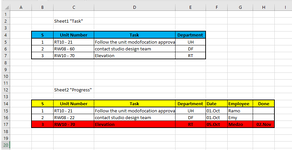
I have two worksheets, sheet1 is a table to list tasks with the unit number named "task" and sheet2 is a table to list the task handling progress named "progress" . and i need to color the task row in sheet1 in red if the same task is mentioned in sheet2 and date is mentioned as done in sheet2 as you can see in screenshot

for example in the screenshot (if C2 in "sheet1"= any cell of "C" in "sheet2" and "H2" IS NOTBLANK) then color entire row in "sheet1" in red

So what is the formula that i can use in conditional formatting to do that

 

[etaf]

both workbooks are on my pc desktop

will they BOTH be open ??
only some functions will work with a closed workbook

looking at your link and files - its a lot different to the example - so not sure what sheet reference now or column references you want to use
need an explanation
the file - name progress - has a sheet called data - I'm assuming thats the sheet you want conditional formatting applied to
Column D is the Unit ID
then you have file AUTHS
No idea what yu are trying to match up on that workbook ?????

very confused now, as things have changed a lot frm our original question and example - and so i MAY NOT be able to answer now


countif() and countifs() will not work with closed workbooks according to this

Functions that Can Access Closed Workbooks

When creating a workbook, you can include formulas that reference data stored in other workbooks. Some functions will even allow you to reference data in another workbook that may be closed. This tip looks at which functions can access that other data, and which cannot.

excelribbon.tips.net

so may need to have some lookup -
But as i say all you are doing is checking that the UNIT Number exists in the other sheet - you done seem to care about any particular status - is that correct
Then maybe a LOOKUP function that does work on closed books - with an IFERROR() or ISNUMBER()

 

[Ramadan2512]

will they BOTH be open ??
only some functions will work with a closed workbook

looking at your link and files - its a lot different to the example - so not sure what sheet reference now or column references you want to use
need an explanation
the file - name progress - has a sheet called data - I'm assuming thats the sheet you want conditional formatting applied to
Column D is the Unit ID
then you have file AUTHS
No idea what yu are trying to match up on that workbook ?????

very confused now, as things have changed a lot frm our original question and example - and so i MAY NOT be able to answer now


countif() and countifs() will not work with closed workbooks according to this

Functions that Can Access Closed Workbooks

When creating a workbook, you can include formulas that reference data stored in other workbooks. Some functions will even allow you to reference data in another workbook that may be closed. This tip looks at which functions can access that other data, and which cannot.

excelribbon.tips.net

so may need to have some lookup -
But as i say all you are doing is checking that the UNIT Number exists in the other sheet - you done seem to care about any particular status - is that correct
Then maybe a LOOKUP function that does work on closed books - with an IFERROR() or ISNUMBER()

will they BOTH be open ??

not always both are open at the same time and yes you are right my posted screenshot was just created simple example
in my real sheet "AUTHS" and "Progress" let's say that what I need to change it's row color is this sheet "AUTHS"
So, in "AUTHS" workbook first sheet "District 1" let's say as folows: (IF(C2 =any cell of "Progress workbook" in column "D" and "H" in progress sheet is <>"" then to color the row in AUTHS with selected color

 

[etaf]

this may work
=IFERROR(INDEX([Progress.xlsm]Data'!$H:$H,MATCH(C9,[Progress.xlsm]Data'!$D:$D,0))<>"",FALSE)

if it matches with the value in progress D with C
MATCH(C9,[Progress.xlsm]Data'!$D:$D,0))
then it will return the value in column H
and test to see if thats NOT blank - Ie a Date
(INDEX([Progress.xlsm]Data'!$H:$H,MATCH(C9,[Progress.xlsm]Data'!$D:$D,0))<>""
and then IF it can not find a match in column D for C - it will retunr an error
and the IFERROR will then return a MATCH

I have put the formula in COLUMN A of AUTHS on the dropbox share

you cannot use conditional formatting into other workbooks

so column A is effectively a helper column - can put in any column
and then use that column for conditional formatting the entire ROW

does that work, as i feel there is a lot more to this then just as described

dropbox link file will only be available for a few days

Dropbox

www.dropbox.com

 

[Ramadan2512]

this may work
=IFERROR(INDEX([Progress.xlsm]Data'!$H:$H,MATCH(C9,[Progress.xlsm]Data'!$D:$D,0))<>"",FALSE)

if it matches with the value in progress D with C
MATCH(C9,[Progress.xlsm]Data'!$D:$D,0))
then it will return the value in column H
and test to see if thats NOT blank - Ie a Date
(INDEX([Progress.xlsm]Data'!$H:$H,MATCH(C9,[Progress.xlsm]Data'!$D:$D,0))<>""
and then IF it can not find a match in column D for C - it will retunr an error
and the IFERROR will then return a MATCH

I have put the formula in COLUMN A of AUTHS on the dropbox share

you cannot use conditional formatting into other workbooks

so column A is effectively a helper column - can put in any column
and then use that column for conditional formatting the entire ROW

does that work, as i feel there is a lot more to this then just as described

dropbox link file will only be available for a few days

Dropbox

www.dropbox.com

I really want to thank you so much for your help and being pateint to help me - thanks a million

 

[etaf]

you are welcome , glad to have helped