Formula or VBA code to format certain cells based on the value.

[Seeker2025]

Good day to everyone!

I am looking for a formula that will apply conditional formatting to a certain based on the value in that cell.

I want to create a job pickup time tracker for three shifts in each sheet each day, each with different operators, and upon the duration of the job and the region number of cells to be highlighted.

Example1

Operator-1 picks a 1-hour duration job, and the job is from the UK region

The value I enter is 1-UK1234 were

1 is the 1-hour duration of the job
UK - Is the UK region code
1234 - Is the Job ID which is not standard

Then four cells to be highlighted considering each cell a 15-minute duration.

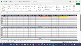
I have also attached the template and given sample data in this and manually highlighted the cells

But I would like to have a VBA code to highlight as many cells depend on the duration and region.

Pls, refer to my attached screenshot. I wanted to attach the excel workbook, but I think only screenshot I can attach.

I want green color for the UK region jobs, Blue for the US region jobs, Orange for the AP region jobs, Yellow for Break, and Red for Leave.

Cheers.

 

[Peter_SSs]

Yes, all the three questions were relevant.

However, my boss has not yet asked for these conditions to be implemented.

It would be a great help if you could also implement those conditions.

or at least questions 2 and 3.

I have looked at all 3 but I have not been able to come up with anything feasible so far for the first case (one job interrupts another job)
Even what I am suggesting below for the second two circumstances may come unstuck.
For example in row 3, if yet another 0.5BR was inserted at, say, column P that would cause the original UK job to spill onto the US job in column T, triggering the first circumstance I asked about earlier and for which my CF is not designed. The CF would fail.
Anyway, see if this is any use for the other two conditions.
With these CF rules, the order is relevant. Enter the bottom one first and work your way up. If they end up in the wrong order you can rearrange them with Conditional Formatting -> Manage Rules by selecting a rule and using the up/down arrows

Seeker2025_2.xlsx
	A	B	C	D	E	F	G	H	I	J	K	L	M	N	O	P	Q	R	S	T	U	V	W	X	Y	Z	AA	AB	AC	AD	AE	AF	AG
3	Name1	3-UK9999			0.5BR				0.5BR			0.25L								0.5-US4563													0.25BR
4	Name2			1.5-US333	0.75L				0.5BR																	1BR
5	Name3		0.5-AP666			1.5-AP4321		1BR
6	Name4	L
7	Name5	L			3-US9999
8	Name6	0.75L			3-US9999
9	Name7
Mon

Cells with Conditional Formatting
Cell	Condition		Cell Format	Stop If True
B3:AG20	Expression	=LET(last,LOOKUP("zzz",$B3:B3),IF(last="L",1,AND(RIGHT(last,1)="L",COLUMNS($B:B)-XMATCH(last,$B3:B3,,-1)<LEFT(last,LEN(last)-1)*4)))	text	NO
B3:AG20	Expression	=LET(last,LOOKUP("zzz",$B3:B3),AND(RIGHT(last,2)="BR",COLUMNS($B:B)-XMATCH(last,$B3:B3,,-1)<LEFT(last,LEN(last)-2)*4))	text	NO
B3:AG20	Expression	=LET(lp,XMATCH("*-UK*",$B3:B3,2,-1),last,INDEX($B3:B3,lp),d,$B3:B3,brl,SUM(--SUBSTITUTE(FILTER(d,(RIGHT(d,2)="BR")*(COLUMN(d)>lp),"0BR"),"BR",""))+SUM(--SUBSTITUTE(FILTER(d,(RIGHT(d,1)="L")*(COLUMN(d)>lp),"0L"),"L","")),AND(COLUMNS($B:B)-lp<(TEXTBEFORE(last,"-")+brl)*4))	text	NO
B3:AG20	Expression	=LET(lp,XMATCH("*-US*",$B3:B3,2,-1),last,INDEX($B3:B3,lp),d,$B3:B3,brl,SUM(--SUBSTITUTE(FILTER(d,(RIGHT(d,2)="BR")*(COLUMN(d)>lp),"0BR"),"BR",""))+SUM(--SUBSTITUTE(FILTER(d,(RIGHT(d,1)="L")*(COLUMN(d)>lp),"0L"),"L","")),AND(COLUMNS($B:B)-lp<(TEXTBEFORE(last,"-")+brl)*4))	text	NO
B3:AG20	Expression	=LET(lp,XMATCH("*-AP*",$B3:B3,2,-1),last,INDEX($B3:B3,lp),d,$B3:B3,brl,SUM(--SUBSTITUTE(FILTER(d,(RIGHT(d,2)="BR")*(COLUMN(d)>lp),"0BR"),"BR",""))+SUM(--SUBSTITUTE(FILTER(d,(RIGHT(d,1)="L")*(COLUMN(d)>lp),"0L"),"L","")),AND(COLUMNS($B:B)-lp<(TEXTBEFORE(last,"-")+brl)*4))	text	NO