summarizing data from multiple tabs in Excel

Harry_1234

New Member
Joined
Aug 19, 2017
Messages
47
I have 28 tabs of data (named AB, BC, CD, EF, FG, GH, HI, IJ, JK, KL, LM, MN, NO, OP, PQ, QR, RS, ST, TU, UV, VW, WX, XY, YZ, Z00, Z01, Z02, Z03) in my spread-sheet with varying data (columns and rows are inconsistent) in each tab. I need a summary tab with count of each column per tab(only should take columns with values into consideration, ignore empty columns) and should be dynamic (i.e. if someone adds an entry into column, the summary tab should update or could click on update to reflect new count). What would be the best way to accomplish this barring pivot tables as i need the flexibility of real-time update. Attached is what i am trying to accomplish?
 

Attachments

  • AB.PNG
    AB.PNG
    26.5 KB · Views: 36
  • BC.PNG
    BC.PNG
    35.2 KB · Views: 36
  • Summary.PNG
    Summary.PNG
    20.7 KB · Views: 36
Time to decide what would be best for the future so that solution ...
- provides a single report of everything required
- and (if necessary) additional options for further flexibility

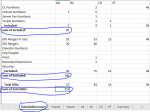
To avoid user confusion ... consider making numbers not in subtotals very obvious!
Items could be marked with an asterisk within current layout (but that is a bit messy) or consider alternative layouts

eg - separate column for excluded items
View attachment 15177

eg - different column for each site with excluded items listed in lower section
(could insert a total column for all sites in Column B)
View attachment 15176

Post a picture if you prefer a different layout

Q Is the same list of headers to be excluded EVERY time, or would you want flexibility to exclude headers of your choosing at time of running report?
Hello,

The second example of having different columns for each site with excluded items listed in lower section is an ideal solution that will perfectly work for me and end users. If i could also have the flexibility to exclude headers of my choice at the time of running report that will be really great. Thanks for all your help until now.
 
Upvote 0

Excel Facts

Whats the difference between CONCAT and CONCATENATE?
The newer CONCAT function can reference a range of cells. =CONCATENATE(A1,A2,A3,A4,A5) becomes =CONCAT(A1:A5)
Put code below in a NEW module and run Summarise2

Please confirm that the VALUES are correct
The code to exclude DID's will be posted later today or tomorrow
VBA Code:
Option Explicit

Private Summary As Worksheet, ws As Worksheet, Cel As Range, x As Long, y As Long
Private Func As WorksheetFunction
Private dID As New Collection, ValidNames As New Collection, Nm As String

Sub Summarise2()
    Application.ScreenUpdating = False
    Call Basics
    Call ValidSheets
    Call WriteColumnA
    Call WriteValues
End Sub
Private Sub Basics()
    Set Summary = Sheets("Summary")
    Set Func = WorksheetFunction
    Summary.Cells.Clear
End Sub
Private Sub ValidSheets()
    Set ValidNames = Nothing
    For Each ws In ThisWorkbook.Worksheets
        Select Case ws.Name
            Case "Summary", "Sheet1", "Check"         '(ignored)
            Case Else:  ValidNames.Add ws.Name
        End Select
    Next ws
End Sub
Private Sub WriteColumnA()
    Set dID = Nothing
        For x = 1 To ValidNames.Count
            On Error Resume Next
            For Each Cel In Sheets(ValidNames(x)).Range("1:1").SpecialCells(xlCellTypeConstants)
                dID.Add Cel.Text, Cel.Text
            Next Cel
            On Error GoTo 0
        Next x
    For x = 1 To dID.Count: Summary.Cells(x + 1, 1) = dID(x): Next
End Sub
Private Sub WriteValues()
    For x = 1 To ValidNames.Count
        Nm = ValidNames(x)
        Summary.Cells(1, x + 1) = Nm
        For y = 1 To dID.Count
            Summary.Cells(y + 1, x + 1) = GetCount(Nm, dID(y))
        Next y
    Next x
    Summary.Cells(1, 1).CurrentRegion.Offset(1).Sort Key1:=Summary.Cells(2, 1), Order1:=xlAscending
End Sub
Private Function GetCount(ByVal shName As String, ByVal idStr As String) As Variant
    Dim c As Long
    On Error Resume Next
    With Sheets(shName)
        c = .Range("1:1").Find(idStr, lookat:=xlWhole).Column
        c = Func.CountA(.Columns(c))
    End With
    If c > 1 Then GetCount = c - 1
    On Error GoTo 0
End Function
 
Last edited:
Upvote 0
Put code below in a NEW module and run Summarise2

Please confirm that the VALUES are correct
The code to exclude DID's will be posted later today or tomorrow
VBA Code:
Option Explicit

Private Summary As Worksheet, ws As Worksheet, Cel As Range, x As Long, y As Long
Private Func As WorksheetFunction
Private dID As New Collection, ValidNames As New Collection, Nm As String

Sub Summarise2()
    Application.ScreenUpdating = False
    Call Basics
    Call ValidSheets
    Call WriteColumnA
    Call WriteValues
End Sub
Private Sub Basics()
    Set Summary = Sheets("Summary")
    Set Func = WorksheetFunction
    Summary.Cells.Clear
End Sub
Private Sub ValidSheets()
    Set ValidNames = Nothing
    For Each ws In ThisWorkbook.Worksheets
        Select Case ws.Name
            Case "Summary", "Sheet1", "Check"         '(ignored)
            Case Else:  ValidNames.Add ws.Name
        End Select
    Next ws
End Sub
Private Sub WriteColumnA()
    Set dID = Nothing
        For x = 1 To ValidNames.Count
            On Error Resume Next
            For Each Cel In Sheets(ValidNames(x)).Range("1:1").SpecialCells(xlCellTypeConstants)
                dID.Add Cel.Text, Cel.Text
            Next Cel
            On Error GoTo 0
        Next x
    For x = 1 To dID.Count: Summary.Cells(x + 1, 1) = dID(x): Next
End Sub
Private Sub WriteValues()
    For x = 1 To ValidNames.Count
        Nm = ValidNames(x)
        Summary.Cells(1, x + 1) = Nm
        For y = 1 To dID.Count
            Summary.Cells(y + 1, x + 1) = GetCount(Nm, dID(y))
        Next y
    Next x
    Summary.Cells(1, 1).CurrentRegion.Offset(1).Sort Key1:=Summary.Cells(2, 1), Order1:=xlAscending
End Sub
Private Function GetCount(ByVal shName As String, ByVal idStr As String) As Variant
    Dim c As Long
    On Error Resume Next
    With Sheets(shName)
        c = .Range("1:1").Find(idStr, lookat:=xlWhole).Column
        c = Func.CountA(.Columns(c))
    End With
    If c > 1 Then GetCount = c - 1
    On Error GoTo 0
End Function
Hello,
Works like a charm. The values are correct.
 
Upvote 0
You may not ultimately want it to run in this exact manner but follow these instructions for the first test

On sheet summary, insert an ActiveX command button
and change its caption to "Run Report
summary command button.jpg


Insert the code below in sheet "Summary" code window
(right click on sheet tab \ View Code \ paste code into that window
VBA Code:
Option Explicit
Const ZZ As String = "ZZ>"        'used in all subs, ZZ used to help with sorting later
Private Sub Worksheet_BeforeRightClick(ByVal Target As Range, Cancel As Boolean)
    If Selection.CountLarge > 1 Then Exit Sub
   
    Dim DIDs As Range: Set DIDs = Range("A1", Range("A" & Rows.Count).End(xlUp).Offset(-1)).Offset(1)
    If Not Intersect(Target, DIDs) Is Nothing Then
        Cancel = True
        Target.Value = ZZ & Target.Value
        Target.Value = Replace(Target.Value, ZZ & ZZ, "")
        Cells(1, 1).Activate
        With DIDs.Resize(, DIDs.CurrentRegion.Columns.Count)
        .Sort Key1:=Cells(2, 2), Order1:=xlAscending
        .Sort Key1:=Cells(2, 1), Order1:=xlAscending
        End With
    End If
End Sub

Private Sub CommandButton1_Click()
    Dim Func As WorksheetFunction: Set Func = WorksheetFunction
    Dim c As Long, r As Long, x As Long, lastC As Long, rng As Range, cel As Range
    Application.ScreenUpdating = False
    Set rng = Sheets("Summary").Range("A1").CurrentRegion
    r = rng.Rows.Count + 1
    lastC = rng.Columns.Count
'copy values to new sheet
    With Sheets.Add(before:=Sheets(1))
        rng.Parent.Cells.Copy
        .Activate
        .Cells.PasteSpecial (xlPasteAll)
        .Cells.PasteSpecial (xlPasteColumnWidths)
        .Cells(1, 1).Select
'add totals
        With .Cells(r, 1).Resize(5)
            .Value = Func.Transpose(Array("   Included:", "", "   Excluded:", "", "   Total DIDs:"))
            .Font.Bold = True
        End With
        For c = 2 To lastC
            .Cells(r + 4, c) = Func.Sum(rng.Columns(c))
            .Cells(r + 2, c) = Func.SumIf(rng.Resize(, 1), ZZ & "*", rng.Columns(c))
            .Cells(r, c) = .Cells(r + 4, c) - .Cells(r + 2, c)
        Next c
'move total to correct line
        On Error Resume Next: x = .Range("A:A").Find(ZZ & "*").Row: On Error GoTo 0
        If x > 0 Then .Rows(r).Resize(2).Cut: .Cells(x, 1).Insert Shift:=xlDown
'remove ZZ
        For Each cel In .Range(rng.Address).Resize(rng.Rows.Count + 2, 1)
            cel.Value = Replace(cel.Value, ZZ, "")
        Next cel
    End With
End Sub

Use right-click to toggle values in column A
ZZ> is auto-inserted in front of items to be excluded (or removed if already listed for exclusion)

summary right-click.jpg


Run Summarise2 to generate the values in sheet "Summary"
(the procedure provided in previous post)

Click on Run Report
report is written to new sheet

summary result.jpg


Click on sheet "Summary"
note : excluded items have not been reset so that you can validate what was selected is correctly transferred to the report
exclude different items and run report again

Let me know how you get on and if there is anything that is not how you want it
 
Upvote 0
You may not ultimately want it to run in this exact manner but follow these instructions for the first test

On sheet summary, insert an ActiveX command button
and change its caption to "Run Report
View attachment 15689

Insert the code below in sheet "Summary" code window
(right click on sheet tab \ View Code \ paste code into that window
VBA Code:
Option Explicit
Const ZZ As String = "ZZ>"        'used in all subs, ZZ used to help with sorting later
Private Sub Worksheet_BeforeRightClick(ByVal Target As Range, Cancel As Boolean)
    If Selection.CountLarge > 1 Then Exit Sub
  
    Dim DIDs As Range: Set DIDs = Range("A1", Range("A" & Rows.Count).End(xlUp).Offset(-1)).Offset(1)
    If Not Intersect(Target, DIDs) Is Nothing Then
        Cancel = True
        Target.Value = ZZ & Target.Value
        Target.Value = Replace(Target.Value, ZZ & ZZ, "")
        Cells(1, 1).Activate
        With DIDs.Resize(, DIDs.CurrentRegion.Columns.Count)
        .Sort Key1:=Cells(2, 2), Order1:=xlAscending
        .Sort Key1:=Cells(2, 1), Order1:=xlAscending
        End With
    End If
End Sub

Private Sub CommandButton1_Click()
    Dim Func As WorksheetFunction: Set Func = WorksheetFunction
    Dim c As Long, r As Long, x As Long, lastC As Long, rng As Range, cel As Range
    Application.ScreenUpdating = False
    Set rng = Sheets("Summary").Range("A1").CurrentRegion
    r = rng.Rows.Count + 1
    lastC = rng.Columns.Count
'copy values to new sheet
    With Sheets.Add(before:=Sheets(1))
        rng.Parent.Cells.Copy
        .Activate
        .Cells.PasteSpecial (xlPasteAll)
        .Cells.PasteSpecial (xlPasteColumnWidths)
        .Cells(1, 1).Select
'add totals
        With .Cells(r, 1).Resize(5)
            .Value = Func.Transpose(Array("   Included:", "", "   Excluded:", "", "   Total DIDs:"))
            .Font.Bold = True
        End With
        For c = 2 To lastC
            .Cells(r + 4, c) = Func.Sum(rng.Columns(c))
            .Cells(r + 2, c) = Func.SumIf(rng.Resize(, 1), ZZ & "*", rng.Columns(c))
            .Cells(r, c) = .Cells(r + 4, c) - .Cells(r + 2, c)
        Next c
'move total to correct line
        On Error Resume Next: x = .Range("A:A").Find(ZZ & "*").Row: On Error GoTo 0
        If x > 0 Then .Rows(r).Resize(2).Cut: .Cells(x, 1).Insert Shift:=xlDown
'remove ZZ
        For Each cel In .Range(rng.Address).Resize(rng.Rows.Count + 2, 1)
            cel.Value = Replace(cel.Value, ZZ, "")
        Next cel
    End With
End Sub

Use right-click to toggle values in column A
ZZ> is auto-inserted in front of items to be excluded (or removed if already listed for exclusion)

View attachment 15688

Run Summarise2 to generate the values in sheet "Summary"
(the procedure provided in previous post)

Click on Run Report
report is written to new sheet

View attachment 15690

Click on sheet "Summary"
note : excluded items have not been reset so that you can validate what was selected is correctly transferred to the report
exclude different items and run report again

Let me know how you get on and if there is anything that is not how you want it
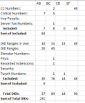
Hello,
Thanks for your quick turnaround and all the help so far. I followed the above instructions and tested the result. All the values have appeared correctly and the exclusion works perfect. There are couple of minor additions I am hoping could be incorporated into this. Can the sum of Included for all sites be included in a separate column below (as shown in screen-shot). Similarly sum of excluded and sum of Total DID's. Also every time I run the report it creates a new sheet, can the same work-sheet be modified with the updated result just like the Summary page. I am open to creating a separate sheet called "DetailedSummary" and have "Run the report" from Summary page transpose results into the "DetailedSummary" sheet every time I run the report. I am just afraid that i might end up with way too many sheets if I don't do the housekeeping.
 

Attachments

  • Sum.PNG
    Sum.PNG
    25.6 KB · Views: 9
Upvote 0
Ensure sheet "DetailedSummary" is in the wokbook before running

Please test code below
As the final step would you prefer everything to happen in the original summary sheet?

VBA Code:
Private Sub CommandButton1_Click()
    Dim Func As WorksheetFunction: Set Func = WorksheetFunction
    Dim c As Long, r As Long, x As Long, lastC As Long, rng As Range, cel As Range
    Application.ScreenUpdating = False
    Set rng = Sheets("Summary").Range("A1").CurrentRegion
    r = rng.Rows.Count + 1
    lastC = rng.Columns.Count
'copy values to new sheet
    With Sheets("DetailedSummary")
        .Cells.Clear
        rng.Parent.Cells.Copy
        .Activate
        .Cells.PasteSpecial (xlPasteAll)
        .Cells.PasteSpecial (xlPasteColumnWidths)
        .Cells(1, 1).Select
'add totals
        With .Cells(r, 1).Resize(8)
            .Value = Func.Transpose(Array("   Included:", "Sum of Included:", "", "   Excluded:", "Sum of Excluded:", "", "   Total DIDs:", "Sum of Total DIDs:"))
            .Font.Bold = True
        End With
        For c = 2 To lastC
            .Cells(r + 6, c) = Func.Sum(rng.Columns(c))
            .Cells(r + 3, c) = Func.SumIf(rng.Resize(, 1), ZZ & "*", rng.Columns(c))
            .Cells(r, c) = .Cells(r + 6, c) - .Cells(r + 3, c)
        Next c
            .Cells(r + 7, 2) = Func.Sum(.Cells(r + 6, 2).Resize(, lastC - 1))
            .Cells(r + 4, 2) = Func.Sum(.Cells(r + 2, 2).Resize(, lastC - 1))
            .Cells(r + 1, 2) = Func.Sum(.Cells(r, 2).Resize(, lastC - 1))
'move total to correct line
        On Error Resume Next: x = .Range("A:A").Find(ZZ & "*").Row: On Error GoTo 0
        If x > 0 Then .Rows(r).Resize(3).Cut: .Cells(x, 1).Insert Shift:=xlDown
'remove XXX
        For Each cel In .Range(rng.Address).Resize(rng.Rows.Count + 5, 1)
            cel.Value = Replace(cel.Value, ZZ, "")
        Next cel
    End With
End Sub
 
Upvote 0
Solution
Ensure sheet "DetailedSummary" is in the wokbook before running

Please test code below
As the final step would you prefer everything to happen in the original summary sheet?

VBA Code:
Private Sub CommandButton1_Click()
    Dim Func As WorksheetFunction: Set Func = WorksheetFunction
    Dim c As Long, r As Long, x As Long, lastC As Long, rng As Range, cel As Range
    Application.ScreenUpdating = False
    Set rng = Sheets("Summary").Range("A1").CurrentRegion
    r = rng.Rows.Count + 1
    lastC = rng.Columns.Count
'copy values to new sheet
    With Sheets("DetailedSummary")
        .Cells.Clear
        rng.Parent.Cells.Copy
        .Activate
        .Cells.PasteSpecial (xlPasteAll)
        .Cells.PasteSpecial (xlPasteColumnWidths)
        .Cells(1, 1).Select
'add totals
        With .Cells(r, 1).Resize(8)
            .Value = Func.Transpose(Array("   Included:", "Sum of Included:", "", "   Excluded:", "Sum of Excluded:", "", "   Total DIDs:", "Sum of Total DIDs:"))
            .Font.Bold = True
        End With
        For c = 2 To lastC
            .Cells(r + 6, c) = Func.Sum(rng.Columns(c))
            .Cells(r + 3, c) = Func.SumIf(rng.Resize(, 1), ZZ & "*", rng.Columns(c))
            .Cells(r, c) = .Cells(r + 6, c) - .Cells(r + 3, c)
        Next c
            .Cells(r + 7, 2) = Func.Sum(.Cells(r + 6, 2).Resize(, lastC - 1))
            .Cells(r + 4, 2) = Func.Sum(.Cells(r + 2, 2).Resize(, lastC - 1))
            .Cells(r + 1, 2) = Func.Sum(.Cells(r, 2).Resize(, lastC - 1))
'move total to correct line
        On Error Resume Next: x = .Range("A:A").Find(ZZ & "*").Row: On Error GoTo 0
        If x > 0 Then .Rows(r).Resize(3).Cut: .Cells(x, 1).Insert Shift:=xlDown
'remove XXX
        For Each cel In .Range(rng.Address).Resize(rng.Rows.Count + 5, 1)
            cel.Value = Replace(cel.Value, ZZ, "")
        Next cel
    End With
End Sub
Tested the code. The sum of Excluded always came out as 0 (see attached screen-shot). Apart from that, the rest worked fine. And yes ideally would prefer everything to happen in original Summary sheet.
 

Attachments

  • SumOfExcluded.PNG
    SumOfExcluded.PNG
    12.6 KB · Views: 8
Upvote 0
oops!
Rich (BB code):
            .Cells(r + 4, 2) = Func.Sum(.Cells(r + 3, 2).Resize(, lastC - 1))
 
Upvote 0

Forum statistics

Threads
1,223,896
Messages
6,175,265
Members
452,627
Latest member
KitkatToby

We've detected that you are using an adblocker.

We have a great community of people providing Excel help here, but the hosting costs are enormous. You can help keep this site running by allowing ads on MrExcel.com.
Allow Ads at MrExcel

Which adblocker are you using?

Disable AdBlock

Follow these easy steps to disable AdBlock

1)Click on the icon in the browser’s toolbar.
2)Click on the icon in the browser’s toolbar.
2)Click on the "Pause on this site" option.
Go back

Disable AdBlock Plus

Follow these easy steps to disable AdBlock Plus

1)Click on the icon in the browser’s toolbar.
2)Click on the toggle to disable it for "mrexcel.com".
Go back

Disable uBlock Origin

Follow these easy steps to disable uBlock Origin

1)Click on the icon in the browser’s toolbar.
2)Click on the "Power" button.
3)Click on the "Refresh" button.
Go back

Disable uBlock

Follow these easy steps to disable uBlock

1)Click on the icon in the browser’s toolbar.
2)Click on the "Power" button.
3)Click on the "Refresh" button.
Go back
Back
Top