Remove blank cell of rows and shift the rest to left

[mehrana]

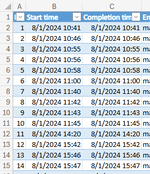
I have a table with 60+ columns. More data is periodically added (using Microsoft form) to this table. There are / will be many blank cells in each row (80% of the entire cells). Instead of this very wide table, I need to display only the data on a screen without the blank cells. The screen can of any kind, such as another table with the blank cells removed and data cells are shifted to left. It will be great if this can done automatically each time when a new row is added or more data is added to cells (on left side of the existing).

I appreciate any help you can provide.

 

[mehrana]

It will update automatically every time the table changes.

That will be great.

I'm a kind of beginner, tried adding the formula a few times, not sure exactly to make it work. Any reference you can possibly provide?

 

[felixstraube]

From your screenshot I asume that you data is in a table.

For the formula to work you need to replace "Table1" with the name of your table.

=LET(t, Table1,
tj, BYROW(t, LAMBDA(x, TEXTJOIN("|", 1, x)&"|")),
res, DROP(REDUCE("", tj, LAMBDA(arr,new, VSTACK(arr, TEXTSPLIT(new, "|")))), 1),
IFERROR(res, "")
)

If you are not sure what the name of the table is you could look in the Name Manager or you could select any cell in the table and go to the menu "Table Design" an look for the Table Name

Let me know if i can help you further.

 

[mehrana]

From your screenshot I asume that you data is in a table.

For the formula to work you need to replace "Table1" with the name of your table.

=LET(t, Table1,
tj, BYROW(t, LAMBDA(x, TEXTJOIN("|", 1, x)&"|")),
res, DROP(REDUCE("", tj, LAMBDA(arr,new, VSTACK(arr, TEXTSPLIT(new, "|")))), 1),
IFERROR(res, "")
)

If you are not sure what the name of the table is you could look in the Name Manager or you could select any cell in the table and go to the menu "Table Design" an look for the Table Name View attachment 114892

Let me know if i can help you further.

Thank you for the hints. I updated your formula with the table's name and added to a new sheet. It is working amazing! the same way I needed.
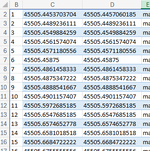
There is only one thing, it converts the data-time date from table like "8/2/2024 1:14:32 PM' to "45506.5517592593". Any idea?

 

[felixstraube]

It is still the same data, it is just formated differently.
if you format the data to date time you should see it correctly.
You could use a conditional formating rule to format it automatically. If you need help with that let me know.

 

[felixstraube]

or use the format painter to copy the format from te original data to the new columns.

 

[mehrana]

or use the format painter to copy the format from te original data to the new columns.

I update the format of new sheet to date/time the same as the sheet1. The format only works correctly outside of the defined region. it does not apply to the column inside.
Format painter sounds like the solution. How can I apply/add that to the formula?

 

[mehrana]

I update the format of new sheet to date/time the same as the sheet1. The format only works correctly outside of the defined region. it does not apply to the column inside.
Format painter sounds like the solution. How can I apply/add that to the formula?

I used Format painter regularly. It only transferred the background color, did not change the data format

 

[felixstraube]

Can you show us what you see?

 

[mehrana]

Can you show us what you see?

Yes, of course. Please see the screenshots, the source sheet (#3) vs the new sheet (#4).

 

[felixstraube]

Try formatting the columns C and D with "dd/mm/yyyy hh:mm"