Help with Excel Text to Column

[Maverick27]

G'Day Excel Gurus

I need help in converting selective cell data from Text to Column.

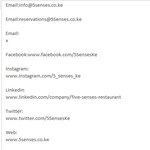
The Column AF data looks the screenshot below:

Anyone care to share a Macro Code (or Excel Function) to convert Text to Column for the following data :

• Email ( 1st instance )
• Facebook
• Instagram
• Web

The Final excel output should look like:

Thanks in Advance.

 

[Alex Blakenburg]

Hi Alex - The Code works like a charm !! Great Stuff !!

Can you pls edit the code to incorporate the data string for Twitter ?

Thanks in Advance.

I have assumed you wanted it in the original order and before Web.

Sub SplitData()

    ' Added Twitter left remarks to assist further additiona

    Dim shtData As Worksheet
    Dim arrSplitCat As Variant
    Dim arrSplitDetail
    Dim lr As Long, i As Long, j  As Long
    Dim rngData As Range, arrData As Variant, rngOut As Range, arrOut As Variant
    Dim iEmail As Long
    
    Set shtData = ActiveSheet
    With shtData
        lr = .Range("AF" & Rows.Count).End(xlUp).Row
        Set rngData = .Range(.Cells(2, "AF"), .Cells(lr, "AF"))
        arrData = rngData
        Set rngOut = .Cells(2, "AG")
    End With
    
    ' Added Twitter - increased column dimension by 1
    ReDim arrOut(1 To UBound(arrData), 1 To 6)
    
    For i = 1 To UBound(arrData)
        iEmail = 1
        arrSplitCat = Split(arrData(i, 1), ";")
        For j = 0 To UBound(arrSplitCat)
            arrSplitDetail = Split(arrSplitCat(j), ":")
            Select Case Trim(arrSplitDetail(0))
            
                Case "Email"
                    If iEmail < 3 Then
                        arrOut(i, iEmail) = Trim(arrSplitDetail(1))
                        iEmail = iEmail + 1
                    End If
                Case "Facebook"
                    arrOut(i, 3) = Trim(arrSplitDetail(1))
                Case "Instagram"
                    arrOut(i, 4) = Trim(arrSplitDetail(1))
                ' Added Twitter - Inserted Case statement
                Case "Twitter"
                    arrOut(i, 5) = Trim(arrSplitDetail(1))
                ' Added Twitter - Since inserted above increased web column by 1
                Case "Web"
                    arrOut(i, 6) = Trim(arrSplitDetail(1))
                Case Else
                    ' do nothing
            End Select
        Next j
    Next i
    
    Set rngOut = rngOut.Resize(UBound(arrOut, 1), UBound(arrOut, 2))
    With rngOut
        .FormulaR1C1 = arrOut
        .Columns.AutoFit
    End With

    Dim rCell As Range
        For Each rCell In rngOut.Resize(, 2)
        shtData.Hyperlinks.Add anchor:=rCell, Address:="mailto:" & rCell.Value
    Next rCell
    
    For Each rCell In rngOut.Offset(, 2).Resize(rngOut.Rows.Count, rngOut.Columns.Count - 2)
        shtData.Hyperlinks.Add anchor:=rCell, Address:="http://" & rCell.Value
    Next rCell

End Sub

 

[Maverick27]

I have assumed you wanted it in the original order and before Web.

Sub SplitData()

    ' Added Twitter left remarks to assist further additiona

    Dim shtData As Worksheet
    Dim arrSplitCat As Variant
    Dim arrSplitDetail
    Dim lr As Long, i As Long, j  As Long
    Dim rngData As Range, arrData As Variant, rngOut As Range, arrOut As Variant
    Dim iEmail As Long
   
    Set shtData = ActiveSheet
    With shtData
        lr = .Range("AF" & Rows.Count).End(xlUp).Row
        Set rngData = .Range(.Cells(2, "AF"), .Cells(lr, "AF"))
        arrData = rngData
        Set rngOut = .Cells(2, "AG")
    End With
   
    ' Added Twitter - increased column dimension by 1
    ReDim arrOut(1 To UBound(arrData), 1 To 6)
   
    For i = 1 To UBound(arrData)
        iEmail = 1
        arrSplitCat = Split(arrData(i, 1), ";")
        For j = 0 To UBound(arrSplitCat)
            arrSplitDetail = Split(arrSplitCat(j), ":")
            Select Case Trim(arrSplitDetail(0))
           
                Case "Email"
                    If iEmail < 3 Then
                        arrOut(i, iEmail) = Trim(arrSplitDetail(1))
                        iEmail = iEmail + 1
                    End If
                Case "Facebook"
                    arrOut(i, 3) = Trim(arrSplitDetail(1))
                Case "Instagram"
                    arrOut(i, 4) = Trim(arrSplitDetail(1))
                ' Added Twitter - Inserted Case statement
                Case "Twitter"
                    arrOut(i, 5) = Trim(arrSplitDetail(1))
                ' Added Twitter - Since inserted above increased web column by 1
                Case "Web"
                    arrOut(i, 6) = Trim(arrSplitDetail(1))
                Case Else
                    ' do nothing
            End Select
        Next j
    Next i
   
    Set rngOut = rngOut.Resize(UBound(arrOut, 1), UBound(arrOut, 2))
    With rngOut
        .FormulaR1C1 = arrOut
        .Columns.AutoFit
    End With

    Dim rCell As Range
        For Each rCell In rngOut.Resize(, 2)
        shtData.Hyperlinks.Add anchor:=rCell, Address:="mailto:" & rCell.Value
    Next rCell
   
    For Each rCell In rngOut.Offset(, 2).Resize(rngOut.Rows.Count, rngOut.Columns.Count - 2)
        shtData.Hyperlinks.Add anchor:=rCell, Address:="http://" & rCell.Value
    Next rCell

End Sub

Thanks Alex !!

 

[Alex Blakenburg]

You're welcome. Glad we could help.