Count And Sum Multiple Columns Grouped on Column

[slipstream]

Hi All,

I've done a search on my problem and come up with many of different solutions but not quite what i need, things like Unique, V/H Stack, Groupby, Index, Match, Sumifs, Countifs, Lookups. TBH it's a little overwhelming I've not used Excel for a long time so bit out of the loop of the advancements.

Hopefully somebody can point me in the right direction.


I'm looking at producing a daily materials plan, data will change daily, however the fields are constant.
I have a Product which has a choice of colour inside, and outside
The inside and outside colours are interchangeable so I don't need to know if a colour is for the inside or outside just quantity per product, however the colours are exclusive to the Product

(I've tried installing XL2BB, however restrictions on the works network are preventing it installing)

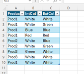
From the attached table, the results expected would be :-

Prod1

White 5​

Blue 2​

Red 2​

Green 1​

​

Prod2

White 2​

Blue 1​

Green 1​

​

Prod3

Green 1​

White 3​

Hopefully, this makes sense, thanks for your time looking.

Product	IntCol	ExtCol
Prod1	White	White
Prod1	White	Green
Prod1	Blue	Blue
Prod1	Red	Red
Prod2	White	Blue
Prod2	White	Green
Prod3	Green	White
Prod3	White	White
Prod1	White	White

 

[slipstream]

Thanks Dave you're a legend

 

[Dave Patton]

There are probably many different approaches to your challenges.
N.B. We do not know the source of your data and we do not know what information you require from the data.
Can you organize the data to expedite preparing useful reports? Long complex formulas can be a challenge to maintain.
Experiment to find the best solutions for you.

T202501a.xlsm
	A	B	C	D	E	F	G	H	I	J	K
1								Count 2 columns
2						Smooth
3	Product	IntCol	ExtCol	Finish			Blue	Green	Red	White	Total
4	Prod1	White	White	Smooth		Prod1			2	4	6
5	Prod1	White	Green	Texture		Prod2	1	1		2	4
6	Prod1	Blue	Blue	Texture		Total	1	1	2	6	10
7	Prod1	Red	Red	Smooth
8	Prod2	White	Blue	Smooth		Texture
9	Prod2	White	Green	Smooth			Blue	Green	White	Total
10	Prod3	Green	White	Texture		Prod1	2	1	1	4
11	Prod3	White	White	Texture		Prod3		1	3	4
12	Prod1	White	White	Smooth		Total	2	2	4	8
13
14
15		IntCol	ExtCol			Smooth|Prod1	Smooth|Prod2	Texture|Prod1	Texture|Prod3	Total
16	Smooth|Prod1	White	White		Blue		1	2		3
17	Texture|Prod1	White	Green		Green		1	1	1	3
18	Texture|Prod1	Blue	Blue		Red	2				2
19	Smooth|Prod1	Red	Red		White	4	2	1	3	10
20	Smooth|Prod2	White	Blue		Total	6	4	4	4	18
21	Smooth|Prod2	White	Green
22	Texture|Prod3	Green	White
23	Texture|Prod3	White	White
24	Smooth|Prod1	White	White
25
26
1cc

Cell Formulas
Range	Formula
F3:K6	F3	=LET(z,FILTER(A4:D12,D4:D12=F2),a,VSTACK(HSTACK(CHOOSECOLS(z,1),CHOOSECOLS(z,2)),HSTACK(CHOOSECOLS(z,1),CHOOSECOLS(z,3))),v,CHOOSECOLS(a,2),PIVOTBY(CHOOSECOLS(a,1),v,v,COUNTA))
F9:J12	F9	=LET(z,FILTER(A4:D12,D4:D12=F8),a,VSTACK(HSTACK(CHOOSECOLS(z,1),CHOOSECOLS(z,2)),HSTACK(CHOOSECOLS(z,1),CHOOSECOLS(z,3))),v,CHOOSECOLS(a,2),PIVOTBY(CHOOSECOLS(a,1),v,v,COUNTA))
E15:J20	E15	=LET(a,VSTACK(A16:B24,HSTACK(A16:A24,C16:C24)),v,CHOOSECOLS(a,2),TRANSPOSE(PIVOTBY(CHOOSECOLS(a,1),v,v,COUNTA)))
A16:A24	A16	=D4&"|"&A4
B16:C24	B16	=B4
Dynamic array formulas.

 

[slipstream]

I've got a source table setup on a worksheet, which will be populated daily with new data, the source data from an external source is formatted for a straight copy and paste.
Then on another worksheet, 2 formatted results tables (=Smooth and =Texture) based on your formula which can be printed giving all the info we need.

It's pretty basic info we need out just wasn't sure on how to group and collate it together, the data format coming in will likely remain constant for sometime so no real need for anything more complex at this point.

It's a little frustrating that I've only got office 2021 at home so can't play around with many of the new functions, just need to find a few spare hours at work to sit down and take a deeper dive.

Many thanks @Dave Patton and the rest of you for spending the time on this for me and giving me a few different avenues to investigate further, much appreciated.

 

[Peter_SSs]

Sorry I'm here again, i'm trying to add a filter to the below, I've added a new column to the table and want to filter depending on criteria.

I've created a filter on it's own and all works fine, =FILTER(Table1,Table1[Finish]="Smooth") however when implementing in to the main formula I'm getting an error.

If you want to keep the table nomenclature (so that the formula automatically adjusts to any increase/decrease in number of data rows) & similar result layout as before ..

slipstream.xlsm
	A	B	C	D	E	F	G	H	I	J	K
1	Product	IntCol	ExtCol	Finish		Finish Filter			Prod1	Prod2	Total
2	Prod1	White	White	Smooth		Smooth		Blue		1	1
3	Prod1	White	Green	Texture				Green		1	1
4	Prod1	Blue	Blue	Texture				Red	2		2
5	Prod1	Red	Red	Smooth				White	4	2	6
6	Prod2	White	Blue	Smooth				Total	6	4	10
7	Prod2	White	Green	Smooth
8	Prod3	Green	White	Texture
9	Prod3	White	White	Texture
10	Prod1	White	White	Smooth
11
12
Sheet1

Cell Formulas
Range	Formula
H1:K6	H1	=LET(f,DROP(FILTER(Table1,Table1[Finish]=F2),,-1),p,TAKE(f,,1),d,HSTACK(VSTACK(p,p),TOCOL(DROP(f,,1),,1)),c,TAKE(d,,-1),TRANSPOSE(PIVOTBY(TAKE(d,,1),c,c,COUNTA)))
Dynamic array formulas.

 

[Peter_SSs]

Two other options if you maybe didn't want that separate filter value cell I have in F2 - but did want the results to reflect what that filter option was ..

1. Put that filter option out of sight, maybe even on another sheet (though I have just put it in column L to demonstrate)

slipstream.xlsm
	A	B	C	D	E	F	G	H	I	J	K	L
1	Product	IntCol	ExtCol	Finish		Smooth	Prod1	Prod2	Total			Finish Filter
2	Prod1	White	White	Smooth		Blue		1	1			Smooth
3	Prod1	White	Green	Texture		Green		1	1
4	Prod1	Blue	Blue	Texture		Red	2		2
5	Prod1	Red	Red	Smooth		White	4	2	6
6	Prod2	White	Blue	Smooth		Total	6	4	10
7	Prod2	White	Green	Smooth
8	Prod3	Green	White	Texture
9	Prod3	White	White	Texture
10	Prod1	White	White	Smooth
11
Sheet1

Cell Formulas
Range	Formula
F1:I6	F1	=LET(f,DROP(FILTER(Table1,Table1[Finish]=L2),,-1),p,TAKE(f,,1),d,HSTACK(VSTACK(p,p),TOCOL(DROP(f,,1),,1)),c,TAKE(d,,-1),a,TRANSPOSE(PIVOTBY(TAKE(d,,1),c,c,COUNTA)),MAKEARRAY(ROWS(a),COLUMNS(a),LAMBDA(r,c,IF(AND(r=1,c=1),L2,INDEX(a,r,c)))))
Dynamic array formulas.

2. Put the filter value in the formula itself but also have it show in the results.

slipstream.xlsm
	A	B	C	D	E	F	G	H	I
1	Product	IntCol	ExtCol	Finish		Smooth	Prod1	Prod2	Total
2	Prod1	White	White	Smooth		Blue		1	1
3	Prod1	White	Green	Texture		Green		1	1
4	Prod1	Blue	Blue	Texture		Red	2		2
5	Prod1	Red	Red	Smooth		White	4	2	6
6	Prod2	White	Blue	Smooth		Total	6	4	10
7	Prod2	White	Green	Smooth
8	Prod3	Green	White	Texture
9	Prod3	White	White	Texture
10	Prod1	White	White	Smooth
11
Sheet1

Cell Formulas
Range	Formula
F1:I6	F1	=LET(flt,"Smooth",f,DROP(FILTER(Table1,Table1[Finish]=flt),,-1),p,TAKE(f,,1),d,HSTACK(VSTACK(p,p),TOCOL(DROP(f,,1),,1)),c,TAKE(d,,-1),a,TRANSPOSE(PIVOTBY(TAKE(d,,1),c,c,COUNTA)),MAKEARRAY(ROWS(a),COLUMNS(a),LAMBDA(r,c,IF(AND(r=1,c=1),flt,INDEX(a,r,c)))))
Dynamic array formulas.

 

[Peter_SSs]

Sorry, yet another thought ..

on another worksheet, 2 formatted results tables (=Smooth and =Texture)

Will the data always have both Finishes or might you need modification along these lines in case not?

slipstream.xlsm
	A	B	C	D	E	F	G
1	Product	IntCol	ExtCol	Finish		No Smooth
2	Prod1	White	White	Texture
3	Prod1	White	Green	Texture
4	Prod1	Blue	Blue	Texture
5	Prod1	Red	Red	Texture
6	Prod2	White	Blue	Texture
7	Prod2	White	Green	Texture
8	Prod3	Green	White	Texture
9	Prod3	White	White	Texture
10	Prod1	White	White	Texture
11
Sheet1

Cell Formulas
Range	Formula
F1	F1	=LET(flt,"Smooth",f,DROP(FILTER(Table1,Table1[Finish]=flt,NA()),,-1),p,TAKE(f,,1),d,HSTACK(VSTACK(p,p),TOCOL(DROP(f,,1),,1)),c,TAKE(d,,-1),a,TRANSPOSE(PIVOTBY(TAKE(d,,1),c,c,COUNTA)),IFNA(MAKEARRAY(ROWS(a),COLUMNS(a),LAMBDA(r,c,IF(AND(r=1,c=1),flt,INDEX(a,r,c)))),"No "&flt))

 

[slipstream]

@Peter_SSs currently it's just the 2 options, either 1 or the other, smooth or texture, later down the line there may be additional, but just the 2 for now.

 

[Peter_SSs]

@Peter_SSs currently it's just the 2 options, either 1 or the other, smooth or texture, later down the line there may be additional, but just the 2 for now.

I think that you may have misinterpreted what I was saying. I didn't mention anything about more then 2 options did I?

 

[slipstream]

Apologies @Peter_SSs , if you're meaning from the source data, then there would always be products with a Smooth Finish, some days would be both and some days there may not be any Texture at all.

 

[Peter_SSs]

some days there may not be any Texture at all.

That is what I was getting at. You has said ..

Then on another worksheet, 2 formatted results tables (=Smooth and =Texture) based on your formula which can be printed

.. and I presumed that if there was no rows with one of Smooth or Texture then you would probably not want #CALC! printed out but either nothing at all for that table or a message indicating no results.
In the mini sheet below cell F5 has a formula from an earlier post of mine and most, if not all, the previous suggestions would produce such an error if no results exist. The modified formula from post 16 in cell F1 I thought might be better if printed. .. or perhaps you would want nothing at all like in cell F3?

slipstream.xlsm
	A	B	C	D	E	F
1	Product	IntCol	ExtCol	Finish		No Texture
2	Prod1	White	White	Smooth
3	Prod1	White	Green	Smooth
4	Prod1	Blue	Blue	Smooth
5	Prod1	Red	Red	Smooth		#CALC!
6	Prod2	White	Blue	Smooth
7	Prod2	White	Green	Smooth
8	Prod3	Green	White	Smooth
9	Prod3	White	White	Smooth
10	Prod1	White	White	Smooth
11
Sheet1

Cell Formulas
Range	Formula
F1	F1	=LET(flt,"Texture",f,DROP(FILTER(Table1,Table1[Finish]=flt,NA()),,-1),p,TAKE(f,,1),d,HSTACK(VSTACK(p,p),TOCOL(DROP(f,,1),,1)),c,TAKE(d,,-1),a,TRANSPOSE(PIVOTBY(TAKE(d,,1),c,c,COUNTA)),IFNA(MAKEARRAY(ROWS(a),COLUMNS(a),LAMBDA(r,c,IF(AND(r=1,c=1),flt,INDEX(a,r,c)))),"No "&flt))
F3	F3	=LET(flt,"Texture",f,DROP(FILTER(Table1,Table1[Finish]=flt,NA()),,-1),p,TAKE(f,,1),d,HSTACK(VSTACK(p,p),TOCOL(DROP(f,,1),,1)),c,TAKE(d,,-1),a,TRANSPOSE(PIVOTBY(TAKE(d,,1),c,c,COUNTA)),IFNA(MAKEARRAY(ROWS(a),COLUMNS(a),LAMBDA(r,c,IF(AND(r=1,c=1),flt,INDEX(a,r,c)))),""))
F5	F5	=LET(flt,"Texture",f,DROP(FILTER(Table1,Table1[Finish]=flt),,-1),p,TAKE(f,,1),d,HSTACK(VSTACK(p,p),TOCOL(DROP(f,,1),,1)),c,TAKE(d,,-1),a,TRANSPOSE(PIVOTBY(TAKE(d,,1),c,c,COUNTA)),MAKEARRAY(ROWS(a),COLUMNS(a),LAMBDA(r,c,IF(AND(r=1,c=1),flt,INDEX(a,r,c)))))