Conditional Formatting of VLOOKUP, Newbie in need of assistance.

[BruceW123]

Hi all,

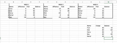
New to the forum. I am a treasurer who needs to track who owes money. As money comes in I fill in names in a speadsheet weekly, which calculates whether someone has paid their weekly fee, or owes money.
I have attached a photo of my excel sheet. I have a VLOOKUP with a column which calculates someone's overall debt. What i would, is a way to conditionally format so that said person's name in the weekly column changes colour to red if they fall below 0 in the bottom right corner where the VLOOKUP table is. Can someone help? Thanks in advance.

 

[etaf]

a countifs may do this for you

something like

countifs($K$11:$K$16, B3, $M$11:$M$16, "<"&0)

Note: Images are difficult to see , and also requires that I input all the data myself, which means I may make an error, which is very time consuming, and from my point of view less likely to get a response, if a complicated spreadsheet. Plus we cannot see any of the formulas used.

Therefore -

A SMALL sample spreadsheet, around 10-20 rows, would help a lot here, with all sensitive data removed, and expected results mocked up and manually entered, with a few notes of explanation.

This will possibly enable a quicker and more accurate solution for you.

MrExcel has a tool called “XL2BB” that lets you post samples of your data and will allow us to copy/paste your sample data into our Excel spreadsheets, saving a lot of time.

XL2BB - Excel Range to BBCode

Excel 'mini-sheet' in messages - XL2BB Although experts prefer to read your description and question instead of working in your actual file to solve your problem, there are times that it is difficult to explain an issue without providing actual...

www.mrexcel.com

You can also test to see if it works ok, in the "Test Here" forum.

Test Here

Use this forum to test your signature, learn bbcode, smilies, XL2BB, etc. Threads in this forum are automatically deleted after no replies for seven (7) days

www.mrexcel.com

OR if you cannot get XL2BB to work, or have restrictions on your PC

then put the sample spreadsheet onto a share

I only tend to goto OneDrive, Dropbox or google docs , as I'm never certain of other random share sites and possible virus.
Please make sure you have a representative data sample and also that the data has been desensitised, remember this site is open to anyone with internet access to see - so any sensitive / personal data should be removed

Make sure you set any share or google to share to everyone

 

[BruceW123]

Book3.xlsx
	A	B	C	D	E	F	G	H	I	J	K	L	M	N
1		WEEK 1				WEEK 2				WEEK 3
2		Name	difference	Paid	Balance	Name	diffeence	Paid	Balance	Name	difference	Paid	Balance
3	1	Tom	0	40		Darryl	10	40		Ben	-30	10
4	2	****	0	40		Harry	0	40		Darryl	0	30
5	3	Harry	0	40		****	-40	0		Harry	0	40
6	4	Darryl	-10	20		Tom	0	40		Tom	10	50
7	5	Ben	-40	0		Ben	-20	20		****	-20	20
8
9
10
11											Name	Charge	Balance
12											Tom	40	10
13											****	40	-60
14											Harry	40	0
15											Ben	40	-90
16											Darryl	30	0
17
18
19
20
21
22
Sheet3

Cell Formulas
Range	Formula
K3,K5:K7,G4:G7,C7,C3:C4	K3	=L3-VLOOKUP(J3,'/Users/talia/Library/CloudStorage/GoogleDrive-siamsaleem@gmail.com/My Drive/Pen Drive/[Falcons Weekly Finances.xlsx]Sheet2'!$A$2:$C$100,2,FALSE)

 

[BruceW123]

Thank you for your assistance. I have downloaded XL2BB and copy and pasted in my sheet. I am not sure if it has worked in its entirety but i hope it has.

 

[BruceW123]

Book3.xlsx
	A	B	C	D	E	F	G	H	I	J	K	L	M	N
1		WEEK 1				WEEK 2				WEEK 3
2		Name	difference	Paid	Balance	Name	diffeence	Paid	Balance	Name	difference	Paid	Balance
3	1	Tom	0	40		Darryl	10	40		Ben	-30	10
4	2	Nick	0	40		Harry	0	40		Darryl	0	30
5	3	Harry	0	40		Nick	40	0		Harry	0	40
6	4	Darryl	-10	20		Tom	0	40		Tom	10	50
7	5	Ben	-40	0		Ben	-20	20		Nick	-20	20
8
9
10
11											Name	Charge	Balance
12											Tom	40	10
13											Nick	40	20
14											Harry	40	0
15											Ben	40	-60
16											Darryl	30	0
17
18
19
20
21
22
23
Sheet3

Cell Formulas
Range	Formula
M12:M16	M12	=SUM(IF(B3:J7=K12, C3:K7,0))

 

[etaf]

I have used =COUNTIFS($K$12:$K$16,B3,$M$12:$M$16,"<"&0) as a conditional formatting rule

for 2007, 2010 , 2013 , 2016 , 2019 or 365 Subscription excel version
Conditional Formatting

Highlight applicable range >>
B3:M7 - Change, reduce or extend the rows to meet your data range of rows

Home Tab >> Styles >> Conditional Formatting
New Rule >> Use a formula to determine which cells to format
Edit the Rule Description: Format values where this formula is true:
=COUNTIFS($K$12:$K$16,B3,$M$12:$M$16,"<"&0)

Format [Number, Font, Border, Fill]
choose the format you would like to apply when the condition is true
OK >> OK

if you also want to highlight the total a simpler conditional format is possible

for 2007, 2010 , 2013 , 2016 , 2019 or 365 Subscription excel version
Conditional Formatting

Highlight applicable range >>
K12:K16 - Change, reduce or extend the rows to meet your data range of rows

Home Tab >> Styles >> Conditional Formatting
New Rule >> Use a formula to determine which cells to format
Edit the Rule Description: Format values where this formula is true:
=M12<0

Format [Number, Font, Border, Fill]
choose the format you would like to apply when the condition is true
OK >> OK

Book1
	A	B	C	D	E	F	G	H	I	J	K	L	M
1		WEEK 1				WEEK 2				WEEK 3
2		Name	difference	Paid	Balance	Name	diffeence	Paid	Balance	Name	difference	Paid	Balance
3	1	Tom	#N/A	40		Darryl	10	40		Ben	#N/A	10
4	2	****	#N/A	40		Harry	#N/A	40		Darryl	0	30
5	3	Harry	0	40		****	#N/A	0		Harry	#N/A	40
6	4	Darryl	-10	20		Tom	#N/A	40		Tom	#N/A	50
7	5	Ben	#N/A	0		Ben	#N/A	20		****	#N/A	20
8
9
10
11											Name	Charge	Balance
12											Tom	40	10
13											****	40	-60
14											Harry	40	0
15											Ben	40	-90
16											Darryl	30	0
Sheet1

Cell Formulas
Range	Formula
K3,K5:K7,G4:G7,C7,C3:C4	K3	=L3-VLOOKUP(J3,'/Users/talia/Library/CloudStorage/GoogleDrive-siamsaleem@gmail.com/My Drive/Pen Drive/[Falcons Weekly Finances.xlsx]Sheet2'!$A$2:$C$100,2,FALSE)

Cells with Conditional Formatting
Cell	Condition		Cell Format	Stop If True
K12:K16	Expression	=M12<0	text	NO
B3:M7	Expression	=COUNTIFS($K$12:$K$16,B3,$M$12:$M$16,"<"&0)	text	NO

 

[BruceW123]

Hi,

Thank you so much for that. I have looked for hours but i think i may have ovecomplicated the matter.

I have one more question. Is there a way to put the table from K12:M16 onto another sheet and use it from there. This way i can put all sensitive info like pricing on sheet 2.

 

[etaf]

yes
but i'm not sure i follow the maths

SUMIFS() will do that for you and you may need to add them together for the different columns

Ben for example shows -90
and has paid 2 lots of 20
when i think 3 lots of 40 due

120 - paid 40 = -80 not -90

anyway i'm not following the maths
and there be better ways to setup up the page ,

or have a running balance

 

[BruceW123]

Hi,

I took out the formulas and the maths didnt add up so i inputted them manually. I have corrected it. Can you show me how to add the lookup table to a separate sheet if possible?

 

[BruceW123]

Booklet 4.xlsx
	A	B	C	D	E	F	G	H	I	J	K	L	M
1		Name	DIFF	Paid	Balance	Name	DIFF	Paid	Balance	Name	DIFF	Paid	Balance
2	1	Tom	-30	10		Ben	10	40		Nick	10	50
3	2	Nick	-20	20		Darryl	0	40		Darryl	0	40
4	3	Harry	-10	30		Nick	15	55		Harry	-10	30
5	4	Darryl	0	40		Harry	-10	30		Ben	-10	20
6	5	Ben	10	40		Tom	-10	30		Tom	-30	10
7
8
9
10
11											Name	Charge	Balance
12											Tom	40	-70
13											Nick	40	5
14											Harry	40	-30
15											Darryl	40	0
16											Ben	30	10
17
Sheet1

Cell Formulas
Range	Formula
C2:C6,K2:K6,G2:G6	C2	=D2-VLOOKUP(B2,$K$12:$M$16, 2,FALSE)
M12:M16	M12	=SUM(IF($B$2:$J$6=K12,$C$2:$K$6,0))

Cells with Conditional Formatting
Cell	Condition		Cell Format	Stop If True
B2:M7	Expression	=COUNTIFS($K$12:$K$20,B2,$M$12:$M$20,"<"&0)	text	NO
B2:M7	Expression	=COUNTIFS($K$12:$K$20,B2,$M$12:$M$20,">"&0)	text	NO