Conditional format help

[khollibygolli]

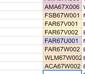
I am trying to highlight duplicates of column C that are SKU product codes on Google Sheets. I currently have =COUNTIF($C$3:C3,C3)>1
My SKUs are 9 characters long but I only want the format to highlight if the 6th-9th characters are a match is this possible?

 

[ChrisFoster]

Take a look at the formula I posted for you just before your last reply.

Did this one work for you Joe? Please test your solutions and try your formulas before posting them

 

[Fluff]

Joe's formula works for me

Fluff.xlsm
	C
1
2
3	E07000125
4	E08000032
5	E08000019
6	E07000198
7	E07000166
8	E08000034
9	E06000047
10	E08000033
11	E07000125
12	E07000030
13	E08000033
14	E08000016
15	E08000019
16	E07000166
17	E07000047
18	E06000052
19	E07000047
20	E07000117
21	E06000049
22	E08000033
23	E06000052
24	E07000125
25	E07000080
26	E08000001
27	E06000047
28	E08000032
29	E08000027
30	E07000007
31	E07000080
32	E07000050
33	E07000037
Main

Cells with Conditional Formatting
Cell	Condition		Cell Format	Stop If True
C3:C33	Expression	=SUMPRODUCT(--(MID(C$3:C3,6,4)=MID(C3,6,4)))>1	text	NO

 

[Joe4]

It didn't work for me . Just made all my blank spaces highlighted

Sounds to me like you are also applying it to blank cells (you did not mention that).
If you want to ignore the blank cells, then try this version:

=SUMPRODUCT(--(C$3:C3<>""),--(MID(C$3:C3,6,4)=MID(C3,6,4)))>1

If that is not working for you, then you may be applying the Conditional Formatting formula incorrectly (many people mix that part up, applying the formula to the correct range).
Tell us what you have done, exactly.

 

[Joe4]

Did this one work for you Joe? Please test your solutions and try your formulas before posting them

Yes, I test my solutions, as should you!
You obviously didn't test mine either!

 

[khollibygolli]

Sounds to me like you are also applying it to blank cells (you did not mention that).
If you want to ignore the blank cells, then try this version:

=SUMPRODUCT(--(C$3:C3<>""),--(MID(C$3:C3,6,4)=MID(C3,6,4)))>1

If that is not working for you, then you may be applying the Conditional Formatting formula incorrectly (many people mix that part up, applying the formula to the correct range).
Tell us what you have done, exactly.

 

[Fluff]

Is this for Excel, or for Google Sheets?

 

[Joe4]

Your "Apply To" range does not coincide with the formula (this is the common mistake that people often make).
You have the formula starting with cell C3, but your "Apply To" range set to C1:C1000.
Change your "Apply To" range to "C3:C1000" and re-enter the formula.

Your Conditional Formatting formula must reflect the very first cell in your "Apply To" range.

 

[khollibygolli]

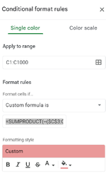
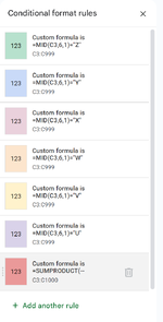
Your "Apply To" range does not coincide with the formula (this is the common mistake that people often make).
You have the formula starting with cell C3, but your "Apply To" range set to C1:C1000.
Change your "Apply To" range to "C3:C1000" and re-enter the formula.

Your Conditional Formatting formula must reflect the very first cell in your "Apply To" range.

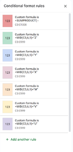
Thank you very much! Not only did I have the C1 C3 wrong but also when having multiple formulas in a column, the order they are arranged matters as well. I moved the sumproduct formula to the top and now it works!!!

 

[Joe4]

You are welcome!
Glad we were able to get it all sorted out.

 

[Fluff]

@khollibygolli can you please confirm if this is for Sheets, Excel or some other app?