Capturing a specific string within another cell...

kbishop94

Active Member
Joined
Dec 5, 2016
Messages
476
Office Version
  1. 365
Platform
  1. Windows
  2. MacOS
I'm trying to figure out a formula that will capture only specific parts of a cells string...

I need a cell in Q to capture specific parts of the adjacent cell to it in column R:
Capture487.JPGCapture488.JPG

I need to capture only the following strings that may (or may not) reside as part of cell R: "CSR21U", "CSR22V", "CSR23W", "CSR24X" or "CSR25Y"

so in the example pics I have shown above, in this particular cell (R18), both CSR23W and CSR24X are present:
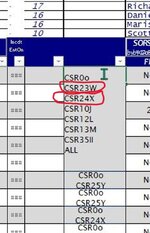
Capture490.JPG

meaning CSR23W and CSR24X would be copied from the target cell and will be displayed in the formula row in cell Q18:
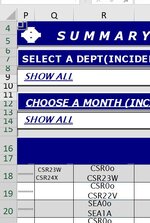
Capture491.JPG

Any help is surely appreciated!!
 

Excel Facts

Copy formula down without changing references
If you have =SUM(F2:F49) in F50; type Alt+' in F51 to copy =SUM(F2:F49) to F51, leaving the formula in edit mode. Change SUM to COUNT.
Could you test this:

Excel Formula:
=TEXTJOIN(CHAR(10),TRUE,BYROW(TRANSPOSE(TEXTSPLIT(R1,CHAR(10))),LAMBDA(a,XLOOKUP(a,F1:F5,F1:F5,""))))

where F1:F5 is your list of values to search, i.e. "CSR21U", "CSR22V", "CSR23W", "CSR24X" or "CSR25Y".
 
Upvote 0
Hi @hagia_sofia
How this LAMBDA(a, works can you please explain.

The TRANSPOSE(TEXTSPLIT(R1,CHAR(10))) part returns an array of individual values; BYROW - LAMBDA(a) provides XLOOKUP with each part of the array (each row) to look for against the list of values.
 
Upvote 0
The merged cells might be problematic. Not sure what you're expecting to return for the sequent rows, but here's an option that returns blanks.
Book1
QR
18CSR23W CSR24XCSR0o CSR23W CSR24X CSR10J CSR12L CSR13M CSR35II ALL
19 
20 
21 
22 
23 
24 
25CSR25YCSR0Oo CSR25Y
Sheet1
Cell Formulas
RangeFormula
Q18:Q25Q18=LET(x,{"CSR21U","CSR22V","CSR23W","CSR24X","CSR25Y"},TEXTJOIN(CHAR(10),,IF(ISNUMBER(SEARCH(x,R18)),x,"")))
 
Upvote 1
Solution
Could you test this:

Excel Formula:
=TEXTJOIN(CHAR(10),TRUE,BYROW(TRANSPOSE(TEXTSPLIT(R1,CHAR(10))),LAMBDA(a,XLOOKUP(a,F1:F5,F1:F5,""))))

where F1:F5 is your list of values to search, i.e. "CSR21U", "CSR22V", "CSR23W", "CSR24X" or "CSR25Y".

Hello hagia_sofia, thank you for your suggestion. However,

Capture492.JPG

I get the dreaded #REF!
Would it have anything to do with how the cell (Q18) is formatted? (I tried some different kinds formats, but to no avail)


But I did have some luck with the suggestion that Cubist offered (shown in cell Q20)
 
Upvote 0
The merged cells might be problematic. Not sure what you're expecting to return for the sequent rows, but here's an option that returns blanks.
Book1
QR
18CSR23W CSR24XCSR0o CSR23W CSR24X CSR10J CSR12L CSR13M CSR35II ALL
19 
20 
21 
22 
23 
24 
25CSR25YCSR0Oo CSR25Y
Sheet1
Cell Formulas
RangeFormula
Q18:Q25Q18=LET(x,{"CSR21U","CSR22V","CSR23W","CSR24X","CSR25Y"},TEXTJOIN(CHAR(10),,IF(ISNUMBER(SEARCH(x,R18)),x,"")))

Thank you Cubist.... your formula and suggestion worked! (see the screen shot shown in my previous reply to hagia_sofia)
also, there are no merged cells involved here. the screen shot just made it look that way ;)
 
Upvote 0
The TRANSPOSE(TEXTSPLIT(R1,CHAR(10))) part returns an array of individual values; BYROW - LAMBDA(a) provides XLOOKUP with each part of the array (each row) to look for against the list of values.

Thanks, but what does "a" does?
 
Upvote 0
Would it have anything to do with how the cell (Q18) is formatted? (I tried some different kinds formats, but to no avail)
You'd need to replace the #REF inside the formula with R18. You must've deleted row 1 at some point.

Thank you Cubist.... your formula and suggestion worked!
You're welcome.
 
Upvote 0
Thanks, but what does "a" does?

When "TRANSPOSE(TEXTSPLIT(R1,CHAR(10)))" is applied, the result is an array of values, e.g. "CSR21U", "CSR22V", "CSR23W", "CSR24X", "CSR25Y"; "a" represents each value of this array and basically says to XLOOKUP search for the first one, then for the second one etc.
 
Upvote 0

Forum statistics

Threads
1,220,965
Messages
6,157,119
Members
451,398
Latest member
rjsteward

We've detected that you are using an adblocker.

We have a great community of people providing Excel help here, but the hosting costs are enormous. You can help keep this site running by allowing ads on MrExcel.com.
Allow Ads at MrExcel

Which adblocker are you using?

Disable AdBlock

Follow these easy steps to disable AdBlock

1)Click on the icon in the browser’s toolbar.
2)Click on the icon in the browser’s toolbar.
2)Click on the "Pause on this site" option.
Go back

Disable AdBlock Plus

Follow these easy steps to disable AdBlock Plus

1)Click on the icon in the browser’s toolbar.
2)Click on the toggle to disable it for "mrexcel.com".
Go back

Disable uBlock Origin

Follow these easy steps to disable uBlock Origin

1)Click on the icon in the browser’s toolbar.
2)Click on the "Power" button.
3)Click on the "Refresh" button.
Go back

Disable uBlock

Follow these easy steps to disable uBlock

1)Click on the icon in the browser’s toolbar.
2)Click on the "Power" button.
3)Click on the "Refresh" button.
Go back
Back
Top