Value from list depending on conditions for Google sheets

[yomarcos]

Hi everyone,

I have been working on this for 2 days straight and I can't figure it out.

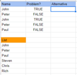
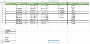
I have a list of employees. Depending on the dates and hours needed for every project I get True or False if there is a conflict. I want a formula that provides me with an alternative when there is a conflict. So in H2 the next option should be James. Thomas is in conflict but Daniel (next on the list) is also in conflict. Please help!!

 

[yomarcos]

Marcelo, you are my new best friend in the whole world.
Thank you?

 

[Marcelo Branco]

You're welcome. Glad to help

M.

 

[yomarcos]

I have 2 more questions!!
Same table without column B (everyone from the same team). How do I do that?
When it gets to the end of the list, I get "". How can I introduce a message in there without adding it to the end of the list?
?

 

[Marcelo Branco]

Didn't understand your question. Please, show a data sample along with expected results

M.

 

[yomarcos]

Sorry!!

There are 2 changes.
1) There is only one team now.
2) When I allocated every employee, I don't have anymore. So I want it to tell me that

 

[Marcelo Branco]

Expected results in G2, G3...???

M.

 

[Marcelo Branco]

Try
=ArrayFormula(IFERROR(IF(--F2=0,"",INDEX(A$13:A$18,SMALL(IF(ISNA(MATCH(A$13:A$18,$E$2:$E$10,0)),ROW(A$13:A$18)-ROW(A$13)+1),COUNTIF(F$2:F2,F2)))),"NOBODY ELSE"))

M.

 

[yomarcos]

Try
=ArrayFormula(IFERROR(IF(--F2=0,"",INDEX(A$13:A$18,SMALL(IF(ISNA(MATCH(A$13:A$18,$E$2:$E$10,0)),ROW(A$13:A$18)-ROW(A$13)+1),COUNTIF(F$2:F2,F2)))),"NOBODY ELSE"))

M.

Thank you!! This is exactly what I needed!!
I tried adding the IFERROR to the previous formula and I failed. Can you please help me again?

 

[Marcelo Branco]

IFERROR should work on any formula even on a Google sheet. Don't know why didnt work for you.

M.

 

[yomarcos]

This worked for me in a Google sheet
H2 copied down
=ArrayFormula(IF(--G2=0;"";INDEX(INDEX(A$13:B$18;0;MATCH(B2;A$12:B$12;0));SMALL(IF(ISNA(MATCH(INDEX(A$13:B$18;0;MATCH(B2;A$12:B$12;0));F$2:F$10;0));ROW(INDEX(A$13:B$18;0;MATCH(B2;A$12:B$12;0)))-ROW(A$13)+1);COUNTIFS(B$2:B2;B2;G$2:G2;G2)))))

M.

Hi Marcelo, This works really well but I found a problem with it. It only goes through the list once. What I mean is, as I mentioned on the original post, Thomas is in conflict but Daniel (next on the list) is also in conflict but when Daniel or Thomas become available again depending on dates, they don't get suggested as alternatives even though there is no conflict