Transposing Info From Columns to Rows - Irregular Pattern

[SimonHughes]

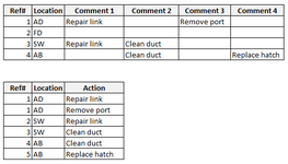
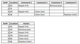
Hello, I have a data set which is in column format and I need to transpose this to row format. There are four columns which could but will not always, have nil, 1, 2 3 or 4 entries and these need to be transposed in rows. The snip below shows original table and the desired outcome. Any help appreciated, many thanks.

Whitbread Remedials Temp.xlsx
	B	C	D	E	F	G
2	Ref#	Location	Comment 1	Comment 2	Comment 3	Comment 4
3	1	AD	Repair link		Remove port
4	2	FD
5	3	SW	Repair link	Clean duct
6	4	AB		Clean duct		Replace hatch
7
8
9	Ref#	Location	Action
10	1	AD	Repair link
11	1	AD	Remove port
12	3	SW	Repair link
13	3	SW	Clean duct
14	4	AB	Clean duct
15	5	AB	Replace hatch
Sheet2

 

[RoryA]

Make the source data into a table, load it into power query, then select the first two columns, right-click a header and choose Unpivot other columns. Job done.

 

[SimonHughes]

Make the source data into a table, load it into power query, then select the first two columns, right-click a header and choose Unpivot other columns. Job done.

Ah, yes, I will need to do a bit of research into Power Query - but it may be worth it, thanks.

 

[RoryA]

it may be worth it

It definitely is - things like this take a couple of minutes.

 

[SimonHughes]

It definitely is - things like this take a couple of minutes.

I am having a play now and will let you know how it goes - later in the day and have to get out now.

 

[footoo]

Here's a macro :

Sub Transpose()

Dim Ws1 As Worksheet: Set Ws1 = Sheets("Sheet1") 'Change as required
Dim Ws2 As Worksheet: Set Ws2 = Sheets("Sheet2") 'Change as required
Dim P1 As Range: Set P1 = Ws1.UsedRange
Dim T1: T1 = P1
Dim T2()
Dim a%: a = 1
Dim i%, j%
ReDim Preserve T2(1 To 3, 1 To a)
T2(1, a) = "Ref#"
T2(2, a) = "Location"
T2(3, a) = "Action"
a = a + 1

For i = 2 To UBound(T1)
    For j = 3 To UBound(T1, 2)
        If T1(i, j) = "" Then GoTo n
        ReDim Preserve T2(1 To 3, 1 To a)
        T2(1, a) = T1(i, 1)
        T2(2, a) = T1(i, 2)
        T2(3, a) = T1(i, j)
        a = a + 1
n:  Next j
Next i

Ws2.[A1].Resize(UBound(T2, 2), UBound(T2)) = Application.Transpose(T2)
End Sub

 

[Peter_SSs]

.. or a formula? (I'm assuming B15 in your mini sheet is an error?)
I have offered two options. The formula in B10 returns the Ref# numbers as Text. If they need to be returned as Numbers then the B18 formula will do that.

24 08 09.xlsm
	B	C	D	E	F	G
2	Ref#	Location	Comment 1	Comment 2	Comment 3	Comment 4
3	1	AD	Repair link		Remove port
4	2	FD
5	3	SW	Repair link	Clean duct
6	4	AB		Clean duct		Replace hatch
7
8
9	Ref#	Location	Action
10	1	AD	Repair link
11	1	AD	Remove port
12	3	SW	Repair link
13	3	SW	Clean duct
14	4	AB	Clean duct
15	4	AB	Replace hatch
16
17
18	1	AD	Repair link
19	1	AD	Remove port
20	3	SW	Repair link
21	3	SW	Clean duct
22	4	AB	Clean duct
23	4	AB	Replace hatch
Cols to Rows

Cell Formulas
Range	Formula
B10:D15	B10	=TEXTSPLIT(TEXTJOIN("#",1,IF(D3:G6="","",B3:B6&"|"&C3:C6&"|"&D3:G6)),"|","#")
B18:D23	B18	=LET(t,TEXTSPLIT(TEXTJOIN("#",1,IF(D3:G6="","",B3:B6&"|"&C3:C6&"|"&D3:G6)),"|","#"),IFERROR(--t,t))
Dynamic array formulas.

 

[JEC]

Two clicks in power query

let
    Source = Excel.CurrentWorkbook(){[Name="Table1"]}[Content],
    unPiv = Table.UnpivotOtherColumns(Source, {"Ref#", "Location"}, "Attribute", "Action"),
    delCol = Table.RemoveColumns(unPiv,{"Attribute"})
in
    delCol

 

[JEC]

Or a formula

=LET(T,C3:F6,HSTACK(TOCOL(IFS(T<>"",A3:A6),2),TOCOL(IFS(T<>"",B3:B6),2),TOCOL(T,1)))

 

[SimonHughes]

.. or a formula? (I'm assuming B15 in your mini sheet is an error?)
I have offered two options. The formula in B10 returns the Ref# numbers as Text. If they need to be returned as Numbers then the B18 formula will do that.

24 08 09.xlsm
	B	C	D	E	F	G
2	Ref#	Location	Comment 1	Comment 2	Comment 3	Comment 4
3	1	AD	Repair link		Remove port
4	2	FD
5	3	SW	Repair link	Clean duct
6	4	AB		Clean duct		Replace hatch
7
8
9	Ref#	Location	Action
10	1	AD	Repair link
11	1	AD	Remove port
12	3	SW	Repair link
13	3	SW	Clean duct
14	4	AB	Clean duct
15	4	AB	Replace hatch
16
17
18	1	AD	Repair link
19	1	AD	Remove port
20	3	SW	Repair link
21	3	SW	Clean duct
22	4	AB	Clean duct
23	4	AB	Replace hatch
Cols to Rows

Cell Formulas
Range	Formula
B10:D15	B10	=TEXTSPLIT(TEXTJOIN("#",1,IF(D3:G6="","",B3:B6&"|"&C3:C6&"|"&D3:G6)),"|","#")
B18:D23	B18	=LET(t,TEXTSPLIT(TEXTJOIN("#",1,IF(D3:G6="","",B3:B6&"|"&C3:C6&"|"&D3:G6)),"|","#"),IFERROR(--t,t))
Dynamic array formulas.

Hi Peter, this formula works well but unfortunately, I have over simplified the example. I have the data on one worksheet and the returns on another. Also, the columns that I want to get returns from are not contiguous. Can I upload a worksheet somehow?