SUMIF slowing calculation times

[OvernightCellebrity]

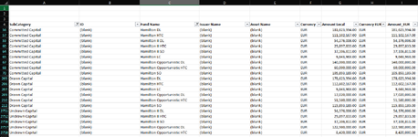
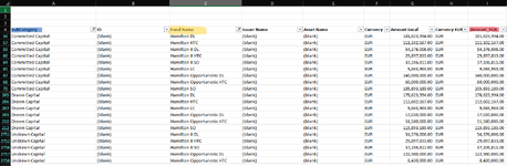
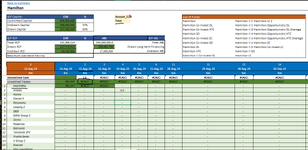
I have the following formula and data (please see images below). How can I improve or modify the formula to avoid slowing down the excel workbook? Note that the sheet contains around 25 tabs an the formula is used multipe times within each tab with various criteria.

I would like to avoid Pivot tables
I cannot change the structure of the underlying data
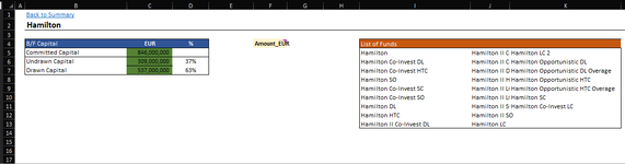
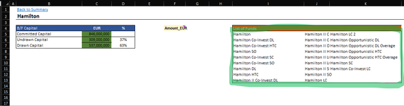
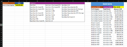
I need the formula to look for every single data point in 'List of funds' see image.

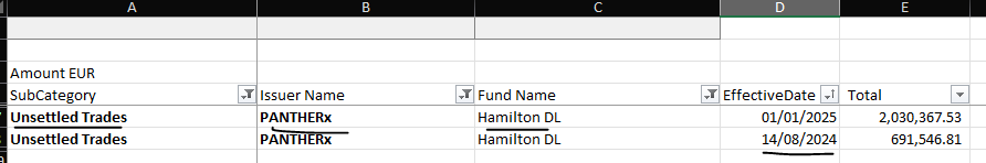
The goal of the formula is to sum/pull/add all values together based on 2 distinct criteria - FUND NAME and Amount_EUR

The problem is the FUND name which has 25 distinct values.

=SUMIFS(INDEX(DailyCash!$G$5:$I$70000,,MATCH($F$4,DailyCash!$G$4:$I$4,0)),DailyCash!$A$5:$A$70000,B5,DailyCash!$C$5:$C$70000,$I$5)+SUMIFS(INDEX(DailyCash!$G$5:$I$70000,,MATCH($F$4,DailyCash!$G$4:$I$4,0)),DailyCash!$A$5:$A$70000,B5,DailyCash!$C$5:$C$70000,$K$10)+SUMIFS(INDEX(DailyCash!$G$5:$I$70000,,MATCH($F$4,DailyCash!$G$4:$I$4,0)),DailyCash!$A$5:$A$70000,B5,DailyCash!$C$5:$C$70000,$I$7)+SUMIFS(INDEX(DailyCash!$G$5:$I$70000,,MATCH($F$4,DailyCash!$G$4:$I$4,0)),DailyCash!$A$5:$A$70000,B5,DailyCash!$C$5:$C$70000,$I$8)+SUMIFS(INDEX(DailyCash!$G$5:$I$70000,,MATCH($F$4,DailyCash!$G$4:$I$4,0)),DailyCash!$A$5:$A$70000,B5,DailyCash!$C$5:$C$70000,$I$9)+SUMIFS(INDEX(DailyCash!$G$5:$I$70000,,MATCH($F$4,DailyCash!$G$4:$I$4,0)),DailyCash!$A$5:$A$70000,B5,DailyCash!$C$5:$C$70000,$I$6)+SUMIFS(INDEX(DailyCash!$G$5:$I$70000,,MATCH($F$4,DailyCash!$G$4:$I$4,0)),DailyCash!$A$5:$A$70000,B5,DailyCash!$C$5:$C$70000,$I$10)+SUMIFS(INDEX(DailyCash!$G$5:$I$70000,,MATCH($F$4,DailyCash!$G$4:$I$4,0)),DailyCash!$A$5:$A$70000,B5,DailyCash!$C$5:$C$70000,$I$11)+SUMIFS(INDEX(DailyCash!$G$5:$I$70000,,MATCH($F$4,DailyCash!$G$4:$I$4,0)),DailyCash!$A$5:$A$70000,B5,DailyCash!$C$5:$C$70000,$I$12)+SUMIFS(INDEX(DailyCash!$G$5:$I$70000,,MATCH($F$4,DailyCash!$G$4:$I$4,0)),DailyCash!$A$5:$A$70000,B5,DailyCash!$C$5:$C$70000,$I$13)+SUMIFS(INDEX(DailyCash!$G$5:$I$70000,,MATCH($F$4,DailyCash!$G$4:$I$4,0)),DailyCash!$A$5:$A$70000,B5,DailyCash!$C$5:$C$70000,$J$5)+SUMIFS(INDEX(DailyCash!$G$5:$I$70000,,MATCH($F$4,DailyCash!$G$4:$I$4,0)),DailyCash!$A$5:$A$70000,B5,DailyCash!$C$5:$C$70000,$J$6)+SUMIFS(INDEX(DailyCash!$G$5:$I$70000,,MATCH($F$4,DailyCash!$G$4:$I$4,0)),DailyCash!$A$5:$A$70000,B5,DailyCash!$C$5:$C$70000,$J$7)+SUMIFS(INDEX(DailyCash!$G$5:$I$70000,,MATCH($F$4,DailyCash!$G$4:$I$4,0)),DailyCash!$A$5:$A$70000,B5,DailyCash!$C$5:$C$70000,$J$8)+SUMIFS(INDEX(DailyCash!$G$5:$I$70000,,MATCH($F$4,DailyCash!$G$4:$I$4,0)),DailyCash!$A$5:$A$70000,B5,DailyCash!$C$5:$C$70000,$J$9)+SUMIFS(INDEX(DailyCash!$G$5:$I$70000,,MATCH($F$4,DailyCash!$G$4:$I$4,0)),DailyCash!$A$5:$A$70000,B5,DailyCash!$C$5:$C$70000,$J$10)+SUMIFS(INDEX(DailyCash!$G$5:$I$70000,,MATCH($F$4,DailyCash!$G$4:$I$4,0)),DailyCash!$A$5:$A$70000,B5,DailyCash!$C$5:$C$70000,$J$11)+SUMIFS(INDEX(DailyCash!$G$5:$I$70000,,MATCH($F$4,DailyCash!$G$4:$I$4,0)),DailyCash!$A$5:$A$70000,B5,DailyCash!$C$5:$C$70000,$J$12)+SUMIFS(INDEX(DailyCash!$G$5:$I$70000,,MATCH($F$4,DailyCash!$G$4:$I$4,0)),DailyCash!$A$5:$A$70000,B5,DailyCash!$C$5:$C$70000,$J$13)+SUMIFS(INDEX(DailyCash!$G$5:$I$70000,,MATCH($F$4,DailyCash!$G$4:$I$4,0)),DailyCash!$A$5:$A$70000,B5,DailyCash!$C$5:$C$70000,$K$5)+SUMIFS(INDEX(DailyCash!$G$5:$I$70000,,MATCH($F$4,DailyCash!$G$4:$I$4,0)),DailyCash!$A$5:$A$70000,B5,DailyCash!$C$5:$C$70000,$K$6)+SUMIFS(INDEX(DailyCash!$G$5:$I$70000,,MATCH($F$4,DailyCash!$G$4:$I$4,0)),DailyCash!$A$5:$A$70000,B5,DailyCash!$C$5:$C$70000,$K$7)+SUMIFS(INDEX(DailyCash!$G$5:$I$70000,,MATCH($F$4,DailyCash!$G$4:$I$4,0)),DailyCash!$A$5:$A$70000,B5,DailyCash!$C$5:$C$70000,$K$8)+SUMIFS(INDEX(DailyCash!$G$5:$I$70000,,MATCH($F$4,DailyCash!$G$4:$I$4,0)),DailyCash!$A$5:$A$70000,B5,DailyCash!$C$5:$C$70000,$K$9)+SUMIFS(INDEX(DailyCash!$G$5:$I$70000,,MATCH($F$4,DailyCash!$G$4:$I$4,0)),DailyCash!$A$5:$A$70000,B5,DailyCash!$C$5:$C$70000,$K$11)

 

[RoryA]

Since you have 365, you could use something like this:

=LET(
dataCol,INDEX(DailyCash!$G$5:$I$70000,,MATCH($F$4,DailyCash!$G$4:$I$4,0)),
crit1,DailyCash!$A$5:$A$70000,
crit2,DailyCash!$C$5:$C$70000,
crit2value,TOCOL($I$5:$K$11,3),
SUM(FILTER(dataCol,MAP(crit1,crit2,LAMBDA(a,b,AND(a=B5,OR(b=crit2value))))))
)

 

[OvernightCellebrity]

Thank you for your response. Please find the revised screenshots attached. I Have added all the data in a single screenshot if easier to visualise the problem ( see

The data I need to extract is in Column `DailyCash!$I$5:$I$70000` (highlighted in red).

The extraction is based on the following criteria:

1. The value in cell `B5` matches the values in Column `DailyCash!$A$5:$A$70000` (highlighted in blue).
2. The values in cells `I5:K25` (highlighted in green) matches the values in Column `DailyCash!$C$5:$C$70000` (highlighted in yellow).

Would the appropriate formula then be?

=LET(DailyCash!$I$5:$I$70000,INDEX(DailyCash!$G$5:$I$70000,,MATCH($F$4,DailyCash!$G$4:$I$4,0)),
I5,DailyCash!$A$5:$A$70000,
I6,DailyCash!$C$5:$C$70000,
I7,TOCOL($I$5:$K$11,3),
SUM(FILTER(dataCol,MAP(I5,I6,LAMBDA(a,b,AND(a=B5,OR(b=crit2value))))))
)

Thank you in advance for the help

 

[RoryA]

No, the formula is exactly what I posted. That is the equivalent of your original formula.

 

[OvernightCellebrity]

THANK YOU!!

 

[kvsrinivasamurthy]

Try this formula.

=LET(a,INDEX(DailyCash!$G$5:$I$17000,,MATCH($F$4,DailyCash!$G$4:$I$4,0)),ro,IF((DailyCash!A5:A17000=B5)*(COUNTIF(I5:K13,DailyCash!C5:C17000)>0),a,""),SUM(ro))

 

[OvernightCellebrity]

One Further question: If i needed to adjust the formula to include additional critical criteria e.g. the date in cell C16 as Crit 3.

AND for the formula to change the source data instead look at 'Pipeline' data sheet - how would i amend the below so that it doesnt return a CALC error 'EMPTY ARRAY'?

Assume it returns this becuase there is no value to find?

=LET(
dataCol, INDEX(Pipeline!$C$4:$E$70000, , MATCH($F$5, Pipeline!$C$4:$E$4, 0)),
crit1, Pipeline!$B$4:$B$70000,
crit2, Pipeline!$C$4:$C$70000,
crit2value, TOCOL($N$5:$P$13, 3),
crit3, Pipeline!$D$4:$D$70000,
SUM(FILTER(dataCol, MAP(crit1, crit2, crit3, LAMBDA(a,b,c, AND(a = B20, OR(b = crit2value), c = C16)))))
)

 

[kvsrinivasamurthy]

Pl try formula in Post#6.
To add criteria Give the date range in DailyCash sheet.

 

[RoryA]

You can return 0 if there is no matching data:

=LET(
dataCol, INDEX(Pipeline!$C$4:$E$70000, , MATCH($F$5, Pipeline!$C$4:$E$4, 0)),
crit1, Pipeline!$B$4:$B$70000,
crit2, Pipeline!$C$4:$C$70000,
crit2value, TOCOL($N$5:$P$13, 3),
crit3, Pipeline!$D$4:$D$70000,
SUM(FILTER(dataCol, MAP(crit1, crit2, crit3, LAMBDA(a,b,c, AND(a = B20, OR(b = crit2value), c = C16))),0))
)

 

[OvernightCellebrity]

Pl try formula in Post#6.
To add criteria Give the date range in DailyCash sheet.

I like the solution in Post 6# but when i apply it to the data in post 7 it returns an #N/A

See formula below

=LET(a,INDEX(Pipeline!$C$4:$E$70000,,MATCH($C$16,Pipeline!$C$4:$E$70000,0)),ro,IF((Pipeline!B4:B70000=B20)*(COUNTIF(N5:P13,Pipeline!$C$4:$C$70000)>0),a,""),SUM(ro))