reverse

[zoharb]

Respected,
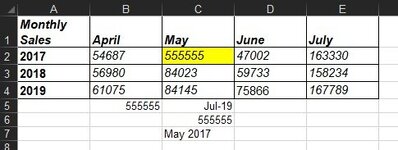
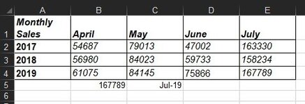
has extracted the MAX value from a list but has to do now reverse thing of finding the month and year when this sales was done.
Thank you in advance
HAPPY NEW YEAR in advance
Zohar Batterywala

EDIT:
jul19 needed in c5 for on basis of max extracted in b5
Zohar Batterywala

 

[Asbestos_Jen]

Does this do what you want?

2024-12-30.xlsx
	A	B	C	D	E
1	Monthly Sales	April	May	June	July
2	2017	54687	79013	47002	163330
3	2018	56980	84023	59733	158234
4	2019	61075	84145	75866	167789
5
6		Max	167789
7		Month	July
8		Year	2019
9		Month & Year	July 2019
Sheet1

Cell Formulas
Range	Formula
C6	C6	=MAX(B2:E4)
C7	C7	=LOOKUP($C$6,B2:E4,B1:E1)
C8	C8	=VLOOKUP($C$6,A1:E4,1)
C9	C9	=C7&" "&C8

 

[Joe4]

Does this do what you want?

2024-12-30.xlsx
	A	B	C	D	E
1	Monthly Sales	April	May	June	July
2	2017	54687	79013	47002	163330
3	2018	56980	84023	59733	158234
4	2019	61075	84145	75866	167789
5
6		Max	167789
7		Month	July
8		Year	2019
9		Month & Year	July 2019
Sheet1

Cell Formulas
Range	Formula
C6	C6	=MAX(B2:E4)
C7	C7	=LOOKUP($C$6,B2:E4,B1:E1)
C8	C8	=VLOOKUP($C$6,A1:E4,1)
C9	C9	=C7&" "&C8

That does not seem to work if the maximum value is not in the last cell.
Here is an example with your formulas when the max is located elsewhere.

The answer should be "June 2018".

 

[zoharb]

Does this do what you want?

2024-12-30.xlsx
	A	B	C	D	E
1	Monthly Sales	April	May	June	July
2	2017	54687	79013	47002	163330
3	2018	56980	84023	59733	158234
4	2019	61075	84145	75866	167789
5
6		Max	167789
7		Month	July
8		Year	2019
9		Month & Year	July 2019
Sheet1

Cell Formulas
Range	Formula
C6	C6	=MAX(B2:E4)
C7	C7	=LOOKUP($C$6,B2:E4,B1:E1)
C8	C8	=VLOOKUP($C$6,A1:E4,1)
C9	C9	=C7&" "&C8

yes this is the answer but I think I will not use it in all other situations.anyway thank you. happy new year

 

[Cubist]

This should work in 2021:

Book1
	A	B	C	D	E
1	Monthly Sales	April	May	June	July
2	2017	54687	79013	9999999	163330
3	2018	56980	5555555	59733	4
4	2019	61075	84145	75866	167789
5
6		Max	9999999
7		Month & Year	June 2017
Sheet1

Cell Formulas
Range	Formula
C6	C6	=MAX(B2:E4)
C7	C7	=CONCAT(IF(C6=B2:E4,B1:E1&" "&A2:A4,""))

 

[zoharb]

This should work in 2021:

Book1
	A	B	C	D	E
1	Monthly Sales	April	May	June	July
2	2017	54687	79013	9999999	163330
3	2018	56980	5555555	59733	4
4	2019	61075	84145	75866	167789
5
6		Max	9999999
7		Month & Year	June 2017
Sheet1

Cell Formulas
Range	Formula
C6	C6	=MAX(B2:E4)
C7	C7	=CONCAT(IF(C6=B2:E4,B1:E1&" "&A2:A4,""))

Respected Sir,
It worked. Thank you VERY VERY MUCH.
Can you please make me understand the logic. PLEASE
Zohar Batterywala

 

[Cubist]

Can you please make me understand the logic

Starting in 2021 with the array functionality added to Excel you can perform binary vector cross product. Some examples:

Book1
	A	B	C	D	E
1	Array 1 * Array 2	1	2	3
2	1	1	2	3
3	2	2	4	6
4	3	3	6	9
5
6	Array 1 ^ Array 2	1	2	3
7	1	1	1	1
8	2	2	4	8
9	3	3	9	27
10
11	Array 1 concats Array 2	April	May	June	July
12	2017	April 2017	May 2017	June 2017	July 2017
13	2018	April 2018	May 2018	June 2018	July 2018
14	2019	April 2019	May 2019	June 2019	July 2019
Sheet2

Cell Formulas
Range	Formula
B2:D4	B2	=A2:A4*B1:D1
B7:D9	B7	=A7:A9^B6:D6
B12:E14	B12	=B11:E11&" " &A12:A14
Dynamic array formulas.

From here, the IF logic returns the concatenated string if it's equal to the MAX, else return empty strings. Finally, CONCAT to reduces the matrix into a single cell (removing the empty strings).

In fact, it'll return all dates with containing the max value. Changed CONCAT to TEXTJOIN for better formatting.

Book1
	A	B	C	D	E
1	Monthly Sales	April	May	June	July
2	2017	54687	79013	5555555	163330
3	2018	56980	5555555	8	4
4	2019	61075	84145	75866	167789
5
6		Max	5555555
7		Month & Year	June 2017, May 2018
Sheet1

Cell Formulas
Range	Formula
C6	C6	=MAX(B2:E4)
C7	C7	=TEXTJOIN(", ",,IF(C6=B2:E4,B1:E1&" "&A2:A4,""))

 

[Arts]

I had no idea Excel could do this. Within your IF formula =CONCAT(IF(C6=B2:E4,B1:E1&" "&A2:A4,"")) I was of the thinking where you have used a range in the true aspect B1:E1&" "&A2:A4 I thought this would return all of the values from B1:E1 and A2:A4 as there was a TRUE value in the range and not just return the true value for that individual cell within the range (hope that makes sense what I'm saying) either way @Cubist very informative and great explanation, thank you.