Return only whole numbers

[riedyp]

Hello ,
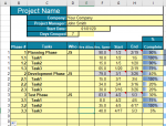
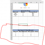
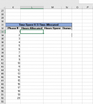
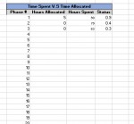
I am trying to make a condensed table(White picture Circled in Red) from returning values in another table(Yellow table). I only want to return the whole numbers without leaving blank spaces. I am currently trying to find the best way to do this. I do not know if its possible to do without VBA. My current method is using the INT function in Column A of the "Yellow picture" to see if column A and B match and then want to return the value of the match to my other table(White Picture" circled in Red) without any spaces between numbers being seen.

 

[KRice]

Could you explain this further, please? I understand the column A and B point, and do not believe that you even need a separate column A, but what is your expectation? The yellow table doesn't show anything in the Hrs Allocated column (col. E), yet for Phase 1 in the white table, 8 hours are shown...same issue for the Hours Spent column, where the yellow table indicates 90 hours for Task 1 and the white table shows only 7. Is your intention to sum all of the hours allocated and spent for each phase (meaning all of the tasks under each phase)? Isn't that already shown in the yellow table where subtotals appear for each phase?

 

[riedyp]

I will also want to return the "Hrs. Allocated" and "Hrs Spent" into that "white table circled red" as well. My intention is to make my "white table circled red" to summarize the "Yellow table" that will be filled out. Meanwhile the "white table circled red" will be locked and unable to be edited. So yes, you were understanding that for the most part.

 

[KRice]

I'm not sure if this is what you have in mind, but have a look at this. There are two sheets: ProjectTasks and ProjectSummary. The ProjectSummary sheet examines column B of the ProjectTask sheet to determine how many main level phases there are, and then it creates a list of those phases (like the 1, 2, and 3 in your white table). Then those phase numbers (in column A of the ProjectSummary worksheet are used with INDEX/MATCH formulas to pull the relevant information from the ProjectTasks worksheet. All of the subtotal work is still done on the ProjectTask worksheet.

Book1c.xlsx
	A	B	C	D	E	F	G	H	I
1		Phase	Tasks	Who	Hrs Alloc	Hrs Spent	Start	End	%Complete
2		1	Planning		80	90			90%
3		1.1	Task 1		8	10
4		1.2	Task 2		12	15
5		1.3	Task 3		60	65
6		2	Dev't		87	79			40%
7		2.1	Task 1		12	15
8		2.2	Task 2		40	34
9		2.3	Task 3		35	30
10		3	Test		90	83			30%
11		3.1	Task 1		10	8
12		3.2	Task 2		30	35
13		3.3	Task 3		50	40
ProjectTasks

Cell Formulas
Range	Formula
E10:F10,E6:F6,E2:F2	E2	=SUBTOTAL(9,E3:E5)

Book1c.xlsx
	A	B	C	D
14	Phase #	Hours Allocated	Hours Spent	Status
15	1	80	90	90%
16	2	87	79	40%
17	3	90	83	30%
18
19
20
21
22
ProjectSummary

Cell Formulas
Range	Formula
A15:A22	A15	=IF(ROW()-ROW(A$14)<=SUMPRODUCT(--(ProjectTasks!$B$2:$B$13=INT(ProjectTasks!$B$2:$B$13))),ROW()-ROW(A$14),"")
B15:B22	B15	=IFERROR(INDEX(ProjectTasks!$B$2:$I$13,MATCH($A15,ProjectTasks!$B$2:$B$13,0),4),"")
C15:C22	C15	=IFERROR(INDEX(ProjectTasks!$B$2:$I$13,MATCH($A15,ProjectTasks!$B$2:$B$13,0),5),"")
D15:D22	D15	=IFERROR(INDEX(ProjectTasks!$B$2:$I$13,MATCH($A15,ProjectTasks!$B$2:$B$13,0),8),"")

 

[riedyp]

Hi Kirk,
Having some trouble with this, below is what i inputted. I am wondering where i am going wrong with this. thank you
K33=IF(ROW()-ROW(A$32)<=SUMPRODUCT(--('Project - Gantt Chart'!$D$9:$D$45 =INT('Project - Gantt Chart'!$D$9:$D$45))),ROW()-ROW(A$32),"")
L33= IFERROR(INDEX('Project - Gantt Chart'!$D$9:$K$45,MATCH('Executive Summary'!$K33,'Project - Gantt Chart'!$D$9:$K$45,0),4),"")
M33=IFERROR(INDEX('Project - Gantt Chart'!$D$9:$K$45,MATCH('Executive Summary'!$K33,'Project - Gantt Chart'!$D$9:$K$45,0),5),"")
N33=IFERROR(INDEX('Project - Gantt Chart'!$D$9:$K$45,MATCH('Executive Summary'!$K33,'Project - Gantt Chart'!$D$9:$K$45,0),8),"")

 

[KRice]

'Project - Gantt Chart'!$D$9:$K$45 should refer to your block of data on the "Project - Gantt Chart" worksheet. If that is correct, then columns D through K represent 8 columns. Can you confirm that you want data returned from the 4th, 5th, and 8th columns (i.e., columns, G, H, and K)?

Did you copy the formula in K33 down into X number or more cells so that the 1st column references can be generated...where X is greater than or equal to the number of main phases on the other sheet?

You can use the XL2BB tool (see links in my signature line or elsewhere on this post) for copying a small portion of your worksheet and uploading it.

 

[KRice]

What did cells K33, L33, M33, and N33 display after you entered those formulas?

 

[riedyp]

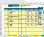
apologies for the confusion i was trying something else but here is my current tables . And yes Phase #'s do show up but that is about it.
With the updated formulas:

K33=IF(ROW()-ROW(A$32)<=SUMPRODUCT(--('Project - Gantt Chart'!$B$9:$B$45 =INT('Project - Gantt Chart'!$B$9:$B$45))),ROW()-ROW(A$32),"")
L33=IFERROR(INDEX('Project - Gantt Chart'!$B$9:$I$45,MATCH('Executive Summary'!$K33,'Project - Gantt Chart'!$B$9:$I$45,0),4),"")
M33=IFERROR(INDEX('Project - Gantt Chart'!$B$9:$I$45,MATCH('Executive Summary'!$K33,'Project - Gantt Chart'!$B$9:$I$45,0),5),"")
N33=IFERROR(INDEX('Project - Gantt Chart'!$B$9:$I$45,MATCH('Executive Summary'!$K33,'Project - Gantt Chart'!$B$9:$I$45,0),8),"")


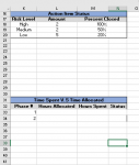
Picture "forum 7" is what happens when i pull down the formula.

 

[KRice]

Try these:

K33=IF(ROW()-ROW(K$32)<=SUMPRODUCT(--('Project - Gantt Chart'!$B$9:$B$45 =INT('Project - Gantt Chart'!$B$9:$B$45))),ROW()-ROW(K$32),"")
L33=IFERROR(INDEX('Project - Gantt Chart'!$B$9:$I$45,MATCH('Executive Summary'!$K33,'Project - Gantt Chart'!$B$9:$B$45,0),4),"")
M33=IFERROR(INDEX('Project - Gantt Chart'!$B$9:$I$45,MATCH('Executive Summary'!$K33,'Project - Gantt Chart'!$B$9:$B$45,0),5),"")
N33=IFERROR(INDEX('Project - Gantt Chart'!$B$9:$I$45,MATCH('Executive Summary'!$K33,'Project - Gantt Chart'!$B$9:$B$45,0),8),"")

You had some issues with your MATCH reference...you want to match the value in column B of the Project-Gantt Chart. Copy all of these across row 33 and then copy down into rows below.

 

[riedyp]

Thank you so much. I should have seen that mistake. Is there anyway for me to format it so that if there are no values for phase 4 then it will not show the number 4? and if there are values in 4 then it will?