Pivot Table - Column is repeating itself with each month - Trend Analysis

[hananak]

Dear All,

I am trying to do Trend analysis on monthly basis for Revenue/Direct cost etc and at the end I put Annual budget. I use Pivot table to do trend analysis. Currently the problem is when I drag Annual budget into value field, the column repeats it self for each month despite being having the same value, as the Annual budget will remain same the whole year.

Is there a way to have the Annual Budget appear only once at the end and not to repeat with each month?

I have the option to either use regular Pivot table or Power Pivot and Power Query or any combination of these, so solution related to any of these will work for me.

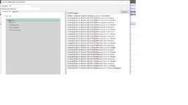
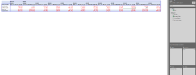
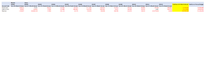
Please see the attached picture to understand the source data structure and the output when I create a pivot table - as you can see the Annual Budget is repeating with each month.

Sorry, on the picture there is a typo - I wanted to write Bottom and instead wrote Button.

Your expert advice would be really appreciated.

 

[hananak]

Would have been good if you had specified that the output had to be a pivot table rather than suggesting it could be anything.

You will need to create a column set for your pivot and remove any columns that show the budget where you don't want them.

Apologise if I was not clear re Pivot table.

Could not understand as I am not allowed to make any changes to source data. All can do is to use power pivot to make changes.

 

[RoryA]

It doesn't involve changing the source data.

then delete the items you don't want:

If you need it to be dynamic, so that it adjusts as new months are added, you will need to edit the MDX directly using the button in the image above, so that it looks something like:

{([Table1].[Months].children,[Measures].[Sum of In Month Actuals]),([Table1].[Months].[All],[Measures].[Sum of In Month Actuals]),([Table1].[Months].[All],[Measures].[Sum of Annual Budget])}

 

[hananak]

It doesn't involve changing the source data.
View attachment 122219

then delete the items you don't want:
View attachment 122220

If you need it to be dynamic, so that it adjusts as new months are added, you will need to edit the MDX directly using the button in the image above, so that it looks something like:

{([Table1].[Months].children,[Measures].[Sum of In Month Actuals]),([Table1].[Months].[All],[Measures].[Sum of In Month Actuals]),([Table1].[Months].[All],[Measures].[Sum of Annual Budget])}

Thanks. The code am seeing on my side is bit different, not sure what to change and where and how many times. Please see the picture I have uploaded.

 

[RoryA]

Yes, you need to replace all of that with what I posted.

 

[hananak]

Yes, you need to replace all of that with what I posted.

Hi, I did replace the code and now the Annual budget is gone completely and it does not allow me to bring any other into Pivot table fields unless I remove the Set. Please see the picture.

 

[RoryA]

Apologies - I didn't look at your pivot table closely enough - you need to enable grand totals for row, since that is where the budget will appear.

 

[hananak]

Apologies - I didn't look at your pivot table closely enough - you need to enable grand totals for row, since that is where the budget will appear.

Thanks. I am getting close to what am desired output is. Can we remove the yellow highlighted part? Rest is fine. It seems like there is restriction to rename the field headings and apply filter on them.

 

[RoryA]

It seems very odd to me that you would not want that shown, but anyway:

{([Table1].[Months].children,[Measures].[Sum of In Month Actuals]),([Table1].[Months].[All],[Measures].[Sum of Annual Budget])}

that version of the MDX should remove that.

 

[hananak]

It seems very odd to me that you would not want that shown, but anyway:

{([Table1].[Months].children,[Measures].[Sum of In Month Actuals]),([Table1].[Months].[All],[Measures].[Sum of Annual Budget])}

that version of the MDX should remove that.

Thank you very much. Now everything is working as I wanted.

I learnt about sets as well which can be quite handy.