Optimization and Filtering

[dsdevon06]

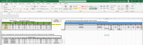
I have two different data sets with similar data but different model numbers. I want to find a discus model that is closest to the reed model based on a certain criteria. That is: Uses the same refrigerant, has the same application, and then the closest capacity. I want this to be robust enough that if the criteria can change. The person who set up this excel previously did not do this. Then once this model is found, it needs outputted in the table to the right with specific data correlating to that discus model.

This was the formula used previously that works but is flawed in its filtering and picking.

=IFERROR(INDEX(A$21:A$25,MATCH(MIN(IF(($E$21:$E$25=$E9)*($C$21:$C$25=$C9)*($I$21:$I$25=$I9)*($J$1=$J$21:$J$25),ABS($G9-$G$21:$G$25))),IF(($E$21:$E$25=$E9)*($J$1=$J$21:$J$25)*($C$21:$C$25=$C9)*($I$21:$I$25=$I9),ABS($G9-$G$21:$G$25)),0)),"-")

Columns M through U and V have similar equations that look through the data set. I tried a pivot table but it gets screwed up with not having exact answers for example, Capacity.

 

[dsdevon06]

I checked what was going on and it was successful.

What about getting the data that correlates to the outputted value

 

[dsdevon06]

Yes. That's what the sortby is doing.


Clear all cells to the right of the formula

Do you need me to share another link?

I am hoping that to the left can it also output the data from the table associated with that row.

 

[Fluff]

That's what the formula does, so not sure what your asking.

 

[dsdevon06]

That's what the formula does, so not sure what your asking.

The formula outputs the two columns worth of data which is J7 and K7. I also need the rest of the data from that row. If J7 was 1AAAA11AA, I would like L7 to be Standard, M7 to be AA1, N7 to be R-11, O7 to be A, P7 to be 11, Q7 to be 1600. I can do the math for R7.

 

[Fluff]

Ok, how about

=LET(f,FILTER(CHOOSECOLS(A$21:J$25,1,2,10,3,4,4,6,7),($E$21:$E$25=$E7)*($D$21:$D$25=$D7)),IFERROR(INDEX(SORTBY(f,ABS(G7-INDEX(f,,7))),1,),"-"))