Matching debit and credit

Ry95

New Member
Joined
May 31, 2024
Messages
6
Office Version
  1. 365
Platform
  1. Windows
Hello,

Its my first real job where i need to use Excel and its lovely but i need some help from real pros.
I need some tips on how to speed up the process off cleaning the sheets, its over 10k rows and im been doing this for almost a month now.
I need to match Debit, Credit and plate number (swedish plates) . On the image plate number abc123 got -7000 and +7000. these need to be removed.
I have been using filters,condition formatting, pivot tables, everything is so slow...

Do you have any tips?
Thanks and sorry for bad english.
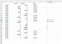
help.PNG.
 

Excel Facts

Difference between two dates
Secret function! Use =DATEDIF(A2,B2,"Y")&" years"&=DATEDIF(A2,B2,"YM")&" months"&=DATEDIF(A2,B2,"MD")&" days"
What if there are 2 credits and 1 debit for the same ID? or 1 credit and 3 debits?
Can you use "Helper columns"?
Does Column A have any significance?
 
Upvote 0
Hello, if there are more credits or debet i need to look up why and manually match or insert from another account.
I tried but its im not so good at finding any shortcuts.
No, its for date. I got columns from A to O but the most importens are Credits,debit and the platenumbers.
 
Upvote 0
This uses a helper column. I added a few extra records for the multiple scenario. Please test it out thoroughly:

Book1
ABCDEFG
1REGHas a Match or Multiple Matches
245300-70000abc1233
34530030659abc1230
44530070000abc1231
545300-16000rae9991
64530016000rae9991
745301-15510
845301-138895KLK0001
945301138895KLK0001
1045302-1753ooo1231
11453021753ooo1231
12453021639400
1345303-4810
1445303-29610
154530070000abc1231
164530070000abc1231
1745303-6429650
1845303-1286950
1945303475995LOk1231
2045303-133995hjh1230
2145303100000hjh1230
2245303-100
2345306-475995LOk1231
Sheet1
Cell Formulas
RangeFormula
G2:G23G2=SUM( (F2=$F$2:$F$23)*(-C2=$D$2:$D$23)*(ISNUMBER(C2))*(C2<>0)+ (F2=$F$2:$F$23)*(-D2=$C$2:$C$23)*(ISNUMBER(D2))*(D2<>0) )


You can also just create a helper column to get the absolute value of the sum of the two columns. Then use AUTOFILTER to sort or use find duplicates:
1719396183417.png


Book1
ABCDEFG
1Dateblank1DebetKredetblank2IDABSOLUTE VALUE
22024-01-0930659abc12330659
32024-01-09-70000abc12370000
42024-01-0970000abc12370000
52024-01-0970000abc12370000
62024-01-0970000abc12370000
72024-01-12100000hjh123100000
82024-01-12-133995hjh123133995
92024-01-10-138895KLK000138895
102024-01-10138895KLK000138895
112024-01-12475995LOk123475995
122024-01-15-475995LOk123475995
132024-01-11-1753ooo1231753
142024-01-111753ooo1231753
152024-01-09-16000rae99916000
162024-01-0916000rae99916000
172024-01-12-1010
182024-01-12-481481
192024-01-10-15511551
202024-01-12-29612961
212024-01-12-128695128695
222024-01-11163940163940
232024-01-12-642965642965
Sheet1
Cell Formulas
RangeFormula
G2:G23G2=ABS(C2+D2)
 
Last edited:
Upvote 0
Solution
Thank you so much, im gonna test it! :)
Have a good day!
 
Upvote 0
Hello again
im trying to change your formula to match this sheet, its almost the same. I tried but keep getting error....
The debit is on I and credit is on J, K and L is for the plate number...
Thanks!

1720689652632.png
 
Upvote 0
My pleasure. Welcome to the forum!
Best Wishes!
Hello again
im trying to change your formula to match this sheet, its almost the same. I tried but keep getting error....
The debit is on I and credit is on J, K and L is for the plate number...
Thanks!

1720689652632.png
 
Upvote 0
Try this. In your first scenario you posted, your KREDITS were negative numbers. In the last post they were not.
Note again, this shows all matches, so the first example has 3 matches, but only one true set of matching Debits and Credits.


Book1
ABCDEFGHIJKLM
1DEBITCREDITTEXTREGHas a Match or Multiple Matches
22024-01-0970000abc1233
32024-01-09306590abc1230
42024-01-09700000abc1231
52024-01-0916000rae9991
62024-01-09160000rae9991
72024-01-1015510
82024-01-10138895KLK0001
92024-01-101388950KLK0001
102024-01-111753ooo1231
112024-01-1117530ooo1231
122024-01-1116394000
132024-01-124810
142024-01-1229610
152024-01-09700000abc1231
162024-01-09700000abc1231
172024-01-126429650
182024-01-121286950
192024-01-124759950LOk1231
202024-01-12133995hjh1230
212024-01-121000000hjh1230
222024-01-12100
232024-01-15475995LOk1231
Sheet4
Cell Formulas
RangeFormula
M2:M23M2=SUM( (L2=$L$2:$L$23)*(I2=$J$2:$J$23)*(ISNUMBER(I2))*(I2<>0)+ (L2=$L$2:$L$23)*(J2=$I$2:$I$23)*(ISNUMBER(J2))*(J2<>0) )
Cells with Conditional Formatting
CellConditionCell FormatStop If True
G2:M23Expression=$M2>0textNO
 
Last edited:
Upvote 0

Forum statistics

Threads
1,223,911
Messages
6,175,324
Members
452,635
Latest member
laura12345

We've detected that you are using an adblocker.

We have a great community of people providing Excel help here, but the hosting costs are enormous. You can help keep this site running by allowing ads on MrExcel.com.
Allow Ads at MrExcel

Which adblocker are you using?

Disable AdBlock

Follow these easy steps to disable AdBlock

1)Click on the icon in the browser’s toolbar.
2)Click on the icon in the browser’s toolbar.
2)Click on the "Pause on this site" option.
Go back

Disable AdBlock Plus

Follow these easy steps to disable AdBlock Plus

1)Click on the icon in the browser’s toolbar.
2)Click on the toggle to disable it for "mrexcel.com".
Go back

Disable uBlock Origin

Follow these easy steps to disable uBlock Origin

1)Click on the icon in the browser’s toolbar.
2)Click on the "Power" button.
3)Click on the "Refresh" button.
Go back

Disable uBlock

Follow these easy steps to disable uBlock

1)Click on the icon in the browser’s toolbar.
2)Click on the "Power" button.
3)Click on the "Refresh" button.
Go back
Back
Top