Macro help

[VBABEGINER]

Hi All, Long back again..

need help in terms of vba code.

I've created one column with the help of Rank formula. Now I want any 2 records of every rank number on another sheet. Randomly. any code can I get please..

 

[VBABEGINER]

You may try such ammended code:

Sub test2()
Dim lr As Long
ActiveSheet.Copy After:=Sheets(1)
ActiveSheet.AutoFilterMode = False
If ActiveSheet.ListObjects.Count > 0 Then ActiveSheet.ListObjects(1).Unlist
lr = Cells(Rows.Count, "BN").End(xlUp).Row
Columns("BQ:BQ").Insert Shift:=xlToRight
Range("BM2:BP" & lr).Sort Key1:=Range("BN2"), Key2:=Range("BP2"), Order2:=xlAscending, Header:=xlNo, Orientation:=xlSortColumns
Range("BQ2:BQ" & lr).FormulaR1C1 = "=COUNTIFS(R1C[-3]:RC[-3],RC[-3],R1C[-1]:RC[-1],""consider"")"
Range("BQ2:BQ" & lr).Value = Range("BQ2:BQ" & lr).Value
Range("BP1:BQ" & lr).AutoFilter Field:=2, Criteria1:="0", Operator:=xlOr, Criteria2:=">2"
Rows("2:" & lr).Delete Shift:=xlUp
ActiveSheet.AutoFilterMode = False
Range("BP1:BQ" & lr).AutoFilter Field:=1, Criteria1:="<>consider"
Rows("2:" & lr).Delete Shift:=xlUp
ActiveSheet.AutoFilterMode = False
Columns("BQ:BQ").Delete Shift:=xlToLeft
End Sub

Hi Kaper, I checked and share some error happening. Could you pls suggest on this..

 

[Kaper]

Of course I have no foggiest idea what ranges were in second CONCAT in column BO. For sure not to the same row. You may convert formulas to values before sorting, as they wil be probably no longer need to be recalculated.

Range("BM2:BP" & lr).value = Range("BM2:BP" & lr).value

would do the job.
so the code would look like:

Sub test3()
Dim lr As Long
ActiveSheet.Copy After:=Sheets(1)
ActiveSheet.AutoFilterMode = False
If ActiveSheet.ListObjects.Count > 0 Then ActiveSheet.ListObjects(1).Unlist
lr = Cells(Rows.Count, "BN").End(xlUp).Row
Columns("BQ:BQ").Insert Shift:=xlToRight
Range("BM2:BP" & lr).value = Range("BM2:BP" & lr).value
Range("BM2:BP" & lr).Sort Key1:=Range("BN2"), Key2:=Range("BP2"), Order2:=xlAscending, Header:=xlNo, Orientation:=xlSortColumns
Range("BQ2:BQ" & lr).FormulaR1C1 = "=COUNTIFS(R1C[-3]:RC[-3],RC[-3],R1C[-1]:RC[-1],""consider"")"
Range("BQ2:BQ" & lr).Value = Range("BQ2:BQ" & lr).Value
Range("BP1:BQ" & lr).AutoFilter Field:=2, Criteria1:="0", Operator:=xlOr, Criteria2:=">2"
Rows("2:" & lr).Delete Shift:=xlUp
ActiveSheet.AutoFilterMode = False
Range("BP1:BQ" & lr).AutoFilter Field:=1, Criteria1:="<>consider"
Rows("2:" & lr).Delete Shift:=xlUp
ActiveSheet.AutoFilterMode = False
Columns("BQ:BQ").Delete Shift:=xlToLeft
End Sub

 

[VBABEGINER]

Of course I have no foggiest idea what ranges were in second CONCAT in column BO. For sure not to the same row. You may convert formulas to values before sorting, as they wil be probably no longer need to be recalculated.

Range("BM2:BP" & lr).value = Range("BM2:BP" & lr).value

would do the job.
so the code would look like:

Sub test3()
Dim lr As Long
ActiveSheet.Copy After:=Sheets(1)
ActiveSheet.AutoFilterMode = False
If ActiveSheet.ListObjects.Count > 0 Then ActiveSheet.ListObjects(1).Unlist
lr = Cells(Rows.Count, "BN").End(xlUp).Row
Columns("BQ:BQ").Insert Shift:=xlToRight
Range("BM2:BP" & lr).value = Range("BM2:BP" & lr).value
Range("BM2:BP" & lr).Sort Key1:=Range("BN2"), Key2:=Range("BP2"), Order2:=xlAscending, Header:=xlNo, Orientation:=xlSortColumns
Range("BQ2:BQ" & lr).FormulaR1C1 = "=COUNTIFS(R1C[-3]:RC[-3],RC[-3],R1C[-1]:RC[-1],""consider"")"
Range("BQ2:BQ" & lr).Value = Range("BQ2:BQ" & lr).Value
Range("BP1:BQ" & lr).AutoFilter Field:=2, Criteria1:="0", Operator:=xlOr, Criteria2:=">2"
Rows("2:" & lr).Delete Shift:=xlUp
ActiveSheet.AutoFilterMode = False
Range("BP1:BQ" & lr).AutoFilter Field:=1, Criteria1:="<>consider"
Rows("2:" & lr).Delete Shift:=xlUp
ActiveSheet.AutoFilterMode = False
Columns("BQ:BQ").Delete Shift:=xlToLeft
End Sub

Hi Kaper, Thank you so much for your reply. I didnt get a chance to cross check the same. I will ensure that either tomorrow EOD or day after tomorrow I will confirm you back.. Till then Thanks again

 

[Kaper]

So, as there was no next post in this thread, probably the solution worked for you. Would be nice if you mark the post with answer (post #12) as a solution.

 

[VBABEGINER]

So, as there was no next post in this thread, probably the solution worked for you. Would be nice if you mark the post with answer (post #12) as a solution.

Hi Kaper, Thanks for your msg. Yesterday only I checked the 2nd solution you provided and i find some difficulty. Hence I did some correction in last column formula make sure that our code will work in much better. will inform you by today.

 

[Kaper]

No problem, I based on "Tomorrow by EOD" declaration in post #13

 

[VBABEGINER]

No problem, I based on "Tomorrow by EOD" declaration in post #13

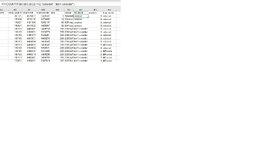
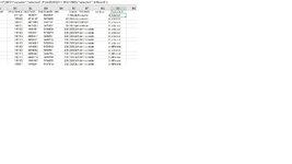
Hi Kaper, can you please do one favor. I've attached few ss. Pls review and can you pls provide me code based on this. what im checking is, if rank is less 2 then it should pick up all those 2 records. If rank count is more than 2 then with the combination of col BN or BO and Col BR, it only gives me 2 records for every record contain in BN or BO.

 

[Fuji]

This will output the results in col.BQ:BR.

Sub test()
    Dim a, b, e, i&, n&, x, y, temp, dic As Object
    Set dic = CreateObject("Scripting.Dictionary")
    a = Range("bm2", Range("bm" & Rows.Count).End(xlUp)(1, 2)).Value
    For i = 1 To UBound(a, 1)
        dic(a(i, 2)) = Trim$(dic(a(i, 2)) & " " & i)
    Next
    ReDim b(1 To dic.Count * 2, 1 To 2)
    For Each e In dic
        x = Split(dic(e))
        If UBound(x) > 1 Then
            For i = 0 To 1
                y = WorksheetFunction.RandBetween(i, UBound(x))
                temp = x(i): x(i) = x(y): x(y) = temp
            Next
        End If
        For i = 0 To 1
            If UBound(x) >= i Then
                n = n + 1
                b(n, 1) = a(x(i), 1): b(n, 2) = a(x(i), 2)
            End If
        Next
    Next
    [bq2].Resize(n, 2) = b
End Sub

 

[VBABEGINER]

Thanks Fuji. I appreciate your time and providing solution to me. Kindly wait, let me check on this.
I also highly appreciate Kaper who as well provides / reply to my post. Thank you Guys, God bless you!

 

[VBABEGINER]

This will output the results in col.BQ:BR.

Sub test()
    Dim a, b, e, i&, n&, x, y, temp, dic As Object
    Set dic = CreateObject("Scripting.Dictionary")
    a = Range("bm2", Range("bm" & Rows.Count).End(xlUp)(1, 2)).Value
    For i = 1 To UBound(a, 1)
        dic(a(i, 2)) = Trim$(dic(a(i, 2)) & " " & i)
    Next
    ReDim b(1 To dic.Count * 2, 1 To 2)
    For Each e In dic
        x = Split(dic(e))
        If UBound(x) > 1 Then
            For i = 0 To 1
                y = WorksheetFunction.RandBetween(i, UBound(x))
                temp = x(i): x(i) = x(y): x(y) = temp
            Next
        End If
        For i = 0 To 1
            If UBound(x) >= i Then
                n = n + 1
                b(n, 1) = a(x(i), 1): b(n, 2) = a(x(i), 2)
            End If
        Next
    Next
    [bq2].Resize(n, 2) = b
End Sub

Hi Fuji, I tested it. Pls refer my ss attached. In col BR it shows which records should be taken (should be consider) but if you see col BN then rows records are the same. Ideally, it shows row records against the number picked up in Col BR. The code only sorts of col BR. Hope did you get what Im trying to explain.

Output ideally comes on different sheet with that numbers you displayed in COl BR. It is perfectly selected but row records of that numbers should also get select