Macro help

[VBABEGINER]

Hi All, Long back again..

need help in terms of vba code.

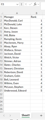
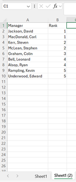
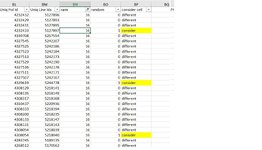
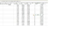
I've created one column with the help of Rank formula. Now I want any 2 records of every rank number on another sheet. Randomly. any code can I get please..

 

[Kaper]

1) assign random number to every record
2) sort records on two keys: 1) rank number 2) assigned random number
3) select only two first records for every rank number

 

[VBABEGINER]

1) assign random number to every record
2) sort records on two keys: 1) rank number 2) assigned random number
3) select only two first records for every rank number

Thank You for your reply. Appreciate the same.
I've the column Rank now. I want a vba code which will do point no 3 you mentioned, on another sheet as output. could you please help on the same. Many Thanks!

 

[Kaper]

Let's assume rank numbers are in column C and random numbers in column D then
3a) in E1 write 1 and in E2 =if(C2<>C1,1,E1+1) and copy down
3b) filter on column E and either
3b1) filter for column E>2 and delete visible, then unfilter
or
3b2) copy only visible data

 

[VBABEGINER]

Let's assume rank numbers are in column C and random numbers in column D then
3a) in E1 write 1 and in E2 =if(C2<>C1,1,E1+1) and copy down
3b) filter on column E and either
3b1) filter for column E>2 and delete visible, then unfilter
or
3b2) copy only visible data

Hi Kaper, Thank You for your reply. Appreciate your effort. But there is something confusion on your logic.
Let me re-explain. I've Rank column with me. What I did is, in power bi table, I used "Rankx" dax on one of the column (i.e. Manager), this will give me unique rank to every Manager.
Suppose, In Manager column manager name is ABC then in power bi Rankx will give rank 1 for this manager. If I've PQR Manager then Rankx will give 2 for this manager. So I took that table output in excel now and my excel have "Rank" column. Now based on these ranks, I only require any 2 records every rank.

Can you give me logic based on my excel output? Many Thanks!

 

[Kaper]

Here is example of the code, for data layout as on attached screenshot:

Sub test()
Dim lr As Long
ActiveSheet.Copy After:=Sheets(1)
lr = Cells(Rows.Count, "A").End(xlUp).Row
Range("C2:C" & lr).Formula = "=RAND()"
Range("A2:C" & lr).Sort Key1:=Range("B2"), Key2:=Range("C2"), Header:=xlNo, Orientation:=xlSortColumns
Range("D2:D" & lr).FormulaR1C1 = "=COUNTIF(R1C[-2]:RC[-2],RC[-2])>2"
Range("A1:D" & lr).AutoFilter Field:=4, Criteria1:="TRUE"
Rows("2:" & lr).Delete Shift:=xlUp
ActiveSheet.AutoFilterMode = False
Columns("C:D").Delete Shift:=xlToLeft
End Sub

Names from Fake Name Generator | HomePage Media
And second screnshot shows the output. Of course every macro run it will be different. PS. I used countif and true/false filtering but of course a formula mentioned in post #4 could be implemented as well (coultif is a bit more intuitive and allows for easier (just a bit) filtering).

 

[VBABEGINER]

Here is example of the code, for data layout as on attached screenshot:

Sub test()
Dim lr As Long
ActiveSheet.Copy After:=Sheets(1)
lr = Cells(Rows.Count, "A").End(xlUp).Row
Range("C2:C" & lr).Formula = "=RAND()"
Range("A2:C" & lr).Sort Key1:=Range("B2"), Key2:=Range("C2"), Header:=xlNo, Orientation:=xlSortColumns
Range("D2:D" & lr).FormulaR1C1 = "=COUNTIF(R1C[-2]:RC[-2],RC[-2])>2"
Range("A1:D" & lr).AutoFilter Field:=4, Criteria1:="TRUE"
Rows("2:" & lr).Delete Shift:=xlUp
ActiveSheet.AutoFilterMode = False
Columns("C:D").Delete Shift:=xlToLeft
End Sub

Names from Fake Name Generator | HomePage Media
And second screnshot shows the output. Of course every macro run it will be different. PS. I used countif and true/false filtering but of course a formula mentioned in post #4 could be implemented as well (coultif is a bit more intuitive and allows for easier (just a bit) filtering).

Thanks for your effort and quick reply. I've changed some logic at my end. Could you please give me code on this logic.

I've attached one screenshot. In Rank column, I've multiple value of that particular rank but I only want to take first 2 records which will "consider" in Col BP. If possible, can you pls help for vba code.

 

[Kaper]

You may try such ammended code:

Sub test2()
Dim lr As Long
ActiveSheet.Copy After:=Sheets(1)
ActiveSheet.AutoFilterMode = False
If ActiveSheet.ListObjects.Count > 0 Then ActiveSheet.ListObjects(1).Unlist
lr = Cells(Rows.Count, "BN").End(xlUp).Row
Columns("BQ:BQ").Insert Shift:=xlToRight
Range("BM2:BP" & lr).Sort Key1:=Range("BN2"), Key2:=Range("BP2"), Order2:=xlAscending, Header:=xlNo, Orientation:=xlSortColumns
Range("BQ2:BQ" & lr).FormulaR1C1 = "=COUNTIFS(R1C[-3]:RC[-3],RC[-3],R1C[-1]:RC[-1],""consider"")"
Range("BQ2:BQ" & lr).Value = Range("BQ2:BQ" & lr).Value
Range("BP1:BQ" & lr).AutoFilter Field:=2, Criteria1:="0", Operator:=xlOr, Criteria2:=">2"
Rows("2:" & lr).Delete Shift:=xlUp
ActiveSheet.AutoFilterMode = False
Range("BP1:BQ" & lr).AutoFilter Field:=1, Criteria1:="<>consider"
Rows("2:" & lr).Delete Shift:=xlUp
ActiveSheet.AutoFilterMode = False
Columns("BQ:BQ").Delete Shift:=xlToLeft
End Sub

 

[VBABEGINER]

You may try such ammended code:

Sub test2()
Dim lr As Long
ActiveSheet.Copy After:=Sheets(1)
ActiveSheet.AutoFilterMode = False
If ActiveSheet.ListObjects.Count > 0 Then ActiveSheet.ListObjects(1).Unlist
lr = Cells(Rows.Count, "BN").End(xlUp).Row
Columns("BQ:BQ").Insert Shift:=xlToRight
Range("BM2:BP" & lr).Sort Key1:=Range("BN2"), Key2:=Range("BP2"), Order2:=xlAscending, Header:=xlNo, Orientation:=xlSortColumns
Range("BQ2:BQ" & lr).FormulaR1C1 = "=COUNTIFS(R1C[-3]:RC[-3],RC[-3],R1C[-1]:RC[-1],""consider"")"
Range("BQ2:BQ" & lr).Value = Range("BQ2:BQ" & lr).Value
Range("BP1:BQ" & lr).AutoFilter Field:=2, Criteria1:="0", Operator:=xlOr, Criteria2:=">2"
Rows("2:" & lr).Delete Shift:=xlUp
ActiveSheet.AutoFilterMode = False
Range("BP1:BQ" & lr).AutoFilter Field:=1, Criteria1:="<>consider"
Rows("2:" & lr).Delete Shift:=xlUp
ActiveSheet.AutoFilterMode = False
Columns("BQ:BQ").Delete Shift:=xlToLeft
End Sub

Hi Kaper, Thanks for your reply and I really appreciate your effort for making my life easy. Thanks again!
I tried the same, but I did get a error, pls refer ss attached.

 

[VBABEGINER]

Hi Kaper, Thanks for your reply and I really appreciate your effort for making my life easy. Thanks again!
I tried the same, but I did get a error, pls refer ss attached.

Hi All, can anyone please help / suggest here a vba code