Lookup nth column value for specified 'n'

Ian McPherson · Aug 9, 2022

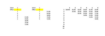
Attached example shows a table of % values. For a specified n=C4 value, lookup up the corresponding %'s from 1-n (yellow highlight).
Thanking you in advance.

Example.xlsx

B

C

D

E

F

G

H

I

J

K

L

M

N

O

P

Q

R

S

T

U

V

W

X

Y

Z

AA

AB

AC

4

Select

21

%

1

2

3

4

5

6

7

8

9

10

11

12

13

14

15

16

17

18

19

20

21

22

5

1

14.0%

1

100.0%

65.0%

50.0%

34.0%

31.0%

25.0%

23.0%

21.0%

20.5%

20.0%

19.0%

18.0%

17.0%

16.0%

15.0%

14.0%

13.0%

6

2

10.0%

2

35.0%

30.0%

28.0%

24.0%

20.0%

19.0%

18.0%

17.0%

16.0%

15.0%

14.0%

13.0%

12.0%

11.0%

10.0%

9.0%

7

3

8.0%

3

20.0%

22.0%

18.0%

17.5%

16.5%

15.0%

14.5%

14.0%

13.0%

12.0%

10.0%

9.0%

8.5%

8.0%

7.8%

8

4

6.6%

4

16.0%

15.0%

14.0%

13.0%

12.0%

11.0%

10.0%

9.0%

8.0%

7.5%

7.0%

6.7%

6.6%

6.5%

9

5

6.0%

5

12.0%

12.5%

11.5%

11.0%

10.0%

9.5%

8.0%

7.0%

6.5%

6.3%

6.2%

6.0%

10

6

5.5%

6

10.0%

9.0%

8.0%

7.0%

6.4%

6.5%

6.0%

5.8%

5.7%

5.5%

11

7

5.0%

7

7.0%

5.5%

6.5%

6.0%

5.8%

5.9%

6.0%

5.5%

5.3%

5.2%

5.0%

12

8

4.6%

8

6.0%

5.0%

5.5%

5.0%

4.9%

5.4%

5.5%

5.0%

4.9%

4.7%

4.6%

13

9

4.2%

9

5.0%

4.5%

4.0%

4.6%

4.5%

5.0%

4.7%

4.6%

4.5%

4.4%

4.2%

14

10

3.9%

10

4.0%

3.8%

3.6%

4.2%

4.6%

4.4%

4.3%

4.1%

3.9%

15

11

3.6%

11

3.2%

3.3%

3.8%

3.9%

4.2%

4.3%

4.2%

4.0%

3.8%

3.6%

16

12

3.4%

12

3.1%

3.4%

3.5%

3.8%

3.9%

3.7%

3.5%

3.6%

3.4%

17

13

3.2%

13

3.0%

3.2%

3.5%

3.6%

3.4%

3.2%

3.4%

3.2%

18

14

3.1%

14

3.0%

3.2%

3.3%

3.2%

3.1%

3.2%

3.1%

19

15

3.0%

15

3.0%

3.1%

3.0%

20

16

2.9%

16

2.8%

3.0%

2.9%

21

17

2.8%

17

2.8%

2.9%

2.8%

22

18

2.7%

18

2.8%

2.7%

23

19

2.6%

19

2.6%

24

20

2.5%

20

2.5%

25

21

2.4%

21

2.4%

26

22

2.3%

Sheet1

Cell Formulas
Range	Formula
C5:C25	C5	=FILTER(G5:G26,(G5:G26<=C4))
Dynamic array formulas.

Cells with Data Validation
Cell	Allow	Criteria
C4	List	=$H$4:$AC$4

Ian McPherson · Oct 3, 2022

As an addition to any of the above formula.....say I input 5 in C4, but then want the 1st % value (31%) to start from (say) the 4th (or any other) position?

Peter_SSs · Oct 4, 2022

Can you give small set of sample data and expected results and explain again in relation to the sample data?

Ian McPherson · Oct 4, 2022

Attached example.
Col D gives the %values corresponding to Col O for the selected integer in C3, using any of the above formulae.
Now I want to introduce a row offset value (G3) which gives the same output (Col H) but offsets the start point by the value G3. If G3 were 0, Col H equals Col D.

Cheers

Peter_SSs · Oct 4, 2022

Ian McPherson said:
Col D gives ...

offset value (G3)

We can't see what is Col D or what id G3

Why not use XL2BB like you did before?

See if you can use (or adapt) this.

Ian McPherson.xlsm

A

B

C

D

E

F

G

H

I

J

K

L

M

N

O

P

Q

R

S

T

U

V

W

X

Y

Z

AA

AB

AC

1

2

3

4

Select

5

%

1

2

3

4

5

6

7

8

9

10

11

12

13

14

15

16

17

18

19

20

21

22

5

Offset

3

1

100.0%

65.0%

50.0%

34.0%

31.0%

25.0%

23.0%

21.0%

20.5%

20.0%

19.0%

18.0%

17.0%

16.0%

15.0%

14.0%

13.0%

6

2

35.0%

30.0%

28.0%

24.0%

20.0%

19.0%

18.0%

17.0%

16.0%

15.0%

14.0%

13.0%

12.0%

11.0%

10.0%

9.0%

7

3

20.0%

22.0%

18.0%

17.5%

16.5%

15.0%

14.5%

14.0%

13.0%

12.0%

10.0%

9.0%

8.5%

8.0%

7.8%

8

4

16.0%

15.0%

14.0%

13.0%

12.0%

11.0%

10.0%

9.0%

8.0%

7.5%

7.0%

6.7%

6.6%

6.5%

9

31.0%

5

12.0%

12.5%

11.5%

11.0%

10.0%

9.5%

8.0%

7.0%

6.5%

6.3%

6.2%

6.0%

10

24.0%

6

10.0%

9.0%

8.0%

7.0%

6.4%

6.5%

6.0%

5.8%

5.7%

5.5%

11

18.0%

7

7.0%

5.5%

6.5%

6.0%

5.8%

5.9%

6.0%

5.5%

5.3%

5.2%

5.0%

12

15.0%

8

6.0%

5.0%

5.5%

5.0%

4.9%

5.4%

5.5%

5.0%

4.9%

4.7%

4.6%

13

12.0%

9

5.0%

4.5%

4.0%

4.6%

4.5%

5.0%

4.7%

4.6%

4.5%

4.4%

4.2%

14

10

4.0%

3.8%

3.6%

4.2%

4.6%

4.4%

4.3%

4.1%

3.9%

15

11

3.2%

3.3%

3.8%

3.9%

4.2%

4.3%

4.2%

4.0%

3.8%

3.6%

16

12

3.1%

3.4%

3.5%

3.8%

3.9%

3.7%

3.5%

3.6%

3.4%

17

13

3.0%

3.2%

3.5%

3.6%

3.4%

3.2%

3.4%

3.2%

18

14

3.0%

3.2%

3.3%

3.2%

3.1%

3.2%

3.1%

19

15

3.0%

3.1%

3.0%

20

16

2.8%

3.0%

2.9%

21

17

2.8%

2.9%

2.8%

22

18

2.8%

2.7%

23

19

2.6%

24

20

2.5%

25

21

2.4%

26

22

2.3%

Extract Col (3)

Cell Formulas
Range	Formula
D5:D13	D5	=VSTACK(TEXTSPLIT(REPT("\|",C5),,"\|"),INDEX(H5:AC26,SEQUENCE(C4),C4))
Dynamic array formulas.

Ian McPherson · Oct 4, 2022

Works well. Can the formula be tweaked for an offset of 0, rather than showing #Value!

Peter_SSs · Oct 4, 2022

Ian McPherson said:
Can the formula be tweaked for an offset of 0, rather than showing #Value!

Can you show us exactly what it would look like with an offset of 0?

Ian McPherson · Oct 4, 2022

See attached

Peter_SSs · Oct 4, 2022

What about this then?

Ian McPherson.xlsm

A

B

C

D

E

F

G

H

I

J

K

L

M

N

1

2

3

4

Select

5

%

1

2

3

4

5

6

7

5

Offset

0

1

100.0%

65.0%

50.0%

34.0%

31.0%

25.0%

23.0%

6

1

31.0%

2

35.0%

30.0%

28.0%

24.0%

20.0%

19.0%

7

2

24.0%

3

20.0%

22.0%

18.0%

17.5%

16.5%

8

3

18.0%

4

16.0%

15.0%

14.0%

9

4

15.0%

5

12.0%

12.5%

11.5%

10

5

12.0%

6

10.0%

9.0%

11

6

7

7.0%

12

7

8

13

8

9

14

10

Extract Col (4)

Cell Formulas
Range	Formula
D5:D10	D5	=VSTACK(IFERROR(TEXTSPLIT(REPT("\|",C5),,"\|"),""),INDEX(H5:AC26,SEQUENCE(C4),C4))
Dynamic array formulas.

Ian McPherson · Oct 4, 2022

That's it! Appreciate your help.

Peter_SSs · Oct 4, 2022

You're welcome. Thanks for confirming.

Lookup nth column value for specified 'n'

Ian McPherson

New Member

Ian McPherson

New Member

Excel Facts

Peter_SSs

MrExcel MVP, Moderator

Ian McPherson

New Member

Attachments

Peter_SSs

MrExcel MVP, Moderator

Ian McPherson

New Member

Peter_SSs

MrExcel MVP, Moderator

Ian McPherson

New Member

Attachments

Peter_SSs

MrExcel MVP, Moderator

Ian McPherson

New Member

Peter_SSs

MrExcel MVP, Moderator

Similar threads

Forum statistics

Share this page

Lookup nth column value for specified 'n'

New Member

New Member

Excel Facts

MrExcel MVP, Moderator

New Member

Attachments

MrExcel MVP, Moderator

New Member

MrExcel MVP, Moderator

New Member

Attachments

MrExcel MVP, Moderator

New Member

MrExcel MVP, Moderator

Similar threads

Forum statistics

Share this page

We've detected that you are using an adblocker.

Which adblocker are you using?

Disable AdBlock

Disable AdBlock Plus

Disable uBlock Origin

Disable uBlock