Lookup Matching Word Within A Sentence

[zakmuh]

Hi All,

I need help with a formula please. I want find the matching word within a sentence (within one cell).

For example:

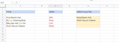
From Column A (A4:A7) 'Ninja Electric Hob', I want to lookup the exact matching word (not partial match) 'Ninja' from Column C (C4:C7) and return the exact matching Title in Column E.

I've attached a screenshot from Excel.

Thanks

Zak

 

[Fluff]

Yeah.

In that case you should make that clear in your initial post, not all Xl functions work in Sheets.
You should also post all Sheets questions in the General Discussion & Other Applications section of the board. I have moved it for you this time.

 

[jtakw]

My guess is that you have "special characters" in your Column A and/or C, are those values downloaded, copy/pasted from somewhere?

 

[zakmuh]

In that case you should make that clear in your initial post, not all Xl functions work in Sheets.
You should also post all Sheets questions in the General Discussion & Other Applications section of the board. I have moved it for you this time.

Thanks for moving and Im sorry about this.

 

[zakmuh]

My guess is that you have "special characters" in your Column A and/or C, are those values downloaded, copy/pasted from somewhere?

It works on Excel but not on google sheet.

Yes I copy pasted from another sheet. I'll try typing them and see if it works. Fingers crossed

 

[zakmuh]

My guess is that you have "special characters" in your Column A and/or C, are those values downloaded, copy/pasted from somewhere?

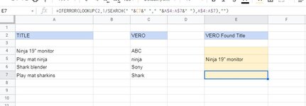
It kinda works in sheet but, its not picking up 'Shark'. Please advise

 

[jtakw]

Even if A6 and C7 is completely deleted, then manually typed over?

 

[zakmuh]

Even if A6 and C7 is completely deleted, then manually typed over?

Yeah, even that didnt work

I tried this formula but this is with 'partial match'. Any suggestions?

=unique(if(isblank(A4:A7),"",(IFERROR(VLOOKUP("*"&C4&"*",A$4:A$7,1,FALSE),""))))

 

[jtakw]

Even if A6 and C7 is completely deleted, then manually typed over?

Yeah, even that didnt work

I tried this formula but this is with 'partial match'. Any suggestions?

=unique(if(isblank(A4:A7),"",(IFERROR(VLOOKUP("*"&C4&"*",A$4:A$7,1,FALSE),""))))

That doesn't sound right, there's something in 1 or both of those cells that's preventing the match.

I don't have the UNIQUE function in 2016, so I can't help with that formula.

 

[Fluff]

Try jtakw's formula like this

=ARRAYFORMULA(IFERROR(LOOKUP(2,1/SEARCH(" "&C4&" "," "&A$4:A$7&" "),A$4:A$7),""))

 

[zakmuh]

Try jtakw's formula like this

=ARRAYFORMULA(IFERROR(LOOKUP(2,1/SEARCH(" "&C4&" "," "&A$4:A$7&" "),A$4:A$7),""))

Nice one It works!

Thanks a lot Fluff and jktaw

I'll apply this to my work and get back to you

Cheers