Isnumber then Vlookup correlating Text and numbers help

[Bthomson]

Hi,

Trying to do something that is WAY too advanced for myself. will try to explain the context of what I need to achieve etc etc.

I have an excel with financial product names in lets say column A
I then have current value of said financial product in Column C
I then have the percentage that they pay for financial product in Column D
and then finally column E is the cost of the current value (So the percentage of the current value)

Current value is always a "-" (dash?) until a numerical value is input

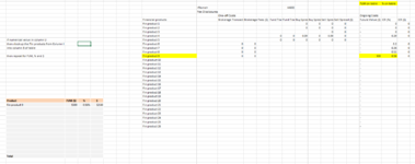
I have a table on a separate sheet that is blank - the table would be as follows

Product name - current value - percentage - Cost

So what I would like to achieve is, ISNumber in column C ? if Yes number, then Vlookup and pull all the product names that have a number in corresponding Current Value

then repeat vlookup to pull all the current values, all the percentages, all the costs into the table

I really have no idea to go about this, standard vlookup is about as advanced as I have been before.

Thanks

 

[bebo021999]

1) You said output table is blank at the beginning. What vlookup_criteria (product name, I guess) shoud be, if it does not exists?

2) Do you refer to get it done via VBA? Its quite easy to trigger change in column C, then update to result table.

 

[Bthomson]

Hey, I have made a sort of mock up of how it looks and tried to explain a little better how I would like it to work.

thanks

 

[bebo021999]

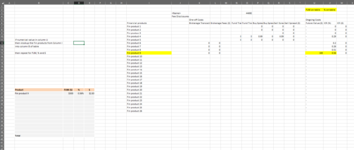
Could you post again with row and column index? We could not see where is column I or U

 

[Alex Blakenburg]

Without Row nos and Column nos it is really hard to give a ready to implement formula.
Your profile says you have MS 365 & 2021 so you should have the filter function.

See if this works for you.

Book4
	A	B	C	D
23	Product	FUM ($)	%	Calc
24	Proj 3	500	0.0056	2.8
25
26
27
Sheet1

Cell Formulas
Range	Formula
A24	A24	=FILTER($I$7:$I$9,ISNUMBER($U$7:$U$9),"")
B24:C24	B24	=FILTER($U$7:$V$9,ISNUMBER($U$7:$U$9),"")
D24	D24	=B24*C24
Dynamic array formulas.

 

[Bthomson]

Sorry, stupid from me haha. have included columns and rows.

 

[Alex Blakenburg]

So in
A27 try this

=FILTER($I$7:$I$40,ISNUMBER($U$7:$U$40),"")

and B27 this

=FILTER($U$7:$V$40,ISNUMBER($U$7:$U$40),"")

 

[Bthomson]

So in
A27 try this

=FILTER($I$7:$I$40,ISNUMBER($U$7:$U$40),"")

and B27 this

=FILTER($U$7:$V$40,ISNUMBER($U$7:$U$40),"")

Didnt work unfortunately, returned value symbol. The data its pulling from is on another tab in the real version of this scenario - so I changed it to correspond to that. frustrating the contents are sensitive info so cant upload the real excel.

 

[Alex Blakenburg]

Start with in A27 typing "=Filter(" then drag and select the rows in the column with your Financial Products in it. Absolute address the selection.
Enter comma then type "Isnumber(" then drag and select the rows in both the FUM $ (should be the same start and end row as in the Fin Products selection) and Absolute address that.
Close with 2 brackets "))".
Then come back to me on the result.