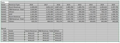
-
If you would like to post, please check out the MrExcel Message Board FAQ and register here. If you forgot your password, you can reset your password.
You are using an out of date browser. It may not display this or other websites correctly.
You should upgrade or use an alternative browser.
You should upgrade or use an alternative browser.
Index with multiple matches (verticle & horizontal)
- Thread starter cshetty
- Start date
MARZIOTULLIO
Well-known Member
- Joined
- Aug 22, 2015
- Messages
- 787
| Book1 | ||||||||||||
|---|---|---|---|---|---|---|---|---|---|---|---|---|
| A | B | C | D | E | F | G | H | I | J | |||
| 1 | Data | |||||||||||
| 2 | Hotel | Revenue Type | 2016 | 2017 | 2018 | 2019 | 2022 | 2023 | 2025 | 2025 | ||
| 3 | Hotel1 | Room Revenue | 2249020 | 2852135 | 2867138 | 2485390 | 1849791 | 1917696 | 2205810 | 2297750 | ||
| 4 | Hotel1 | F&B Revenue -Total | 3839961 | 3717726 | 3660473 | 3647724 | 2652356 | 2832327 | 3168098 | 3696147 | ||
| 5 | Hotel1 | Others | 1020865 | 1252066 | 1131119 | 9432.22 | 690838 | 712683 | 758333 | 849983 | ||
| 6 | Hotel1 | NOP | 1161291 | 1678180 | 1559411 | 1397026 | 1092964 | 1123772 | 1423707 | 1628732 | ||
| 7 | Hotel2 | Room Revenue | 2830586 | 2884414 | 2835441 | 2517192 | 1762052 | 1820568 | 1513673 | 1700501 | ||
| 8 | Hotel2 | F&B Revenue -Total | 2893392 | 2818648 | 2886624 | 2639726 | 2113070 | 2086827 | 1966306 | 2040472 | ||
| 9 | Hotel2 | Others | 619152 | 684913 | 702274 | 658191 | 603993 | 624001 | 643444 | 642028 | ||
| 10 | ||||||||||||
| 11 | Result | |||||||||||
| 12 | Year | Hotel | Room Revenue | F&B Revenue -Total | Others | |||||||
| 13 | 2016 | Hotel1 | 2249020 | 3839961 | 1020865 | |||||||
| 14 | 2016 | Hotel2 | 2830586 | 2893392 | 619152 | |||||||
| 15 | 2017 | Hotel1 | 2852135 | 3717726 | 1252066 | |||||||
| 16 | 2017 | Hotel2 | 2884414 | 2818648 | 684913 | |||||||
Sheet2 | ||||||||||||
| Cell Formulas | ||
|---|---|---|
| Range | Formula | |
| C13:E16 | C13 | =SUMIFS(INDEX($C$3:$J$9,,MATCH($A13,$C$2:$J$2,0)),$A$3:$A$9,$B13,$B$3:$B$9,C$12) |
copy across and down
Upvote
0
Peter_SSs
MrExcel MVP, Moderator
- Joined
- May 28, 2005
- Messages
- 65,932
- Office Version
- 365
- Platform
- Windows
To tune your formula, try this very small change (in your version you may need to confirm it with Ctrl+Shift+Enter, not just Enter)Please help me to tune this formula.
=INDEX($F$4:$M$10,MATCH(1,($E15=$D$4:$D$10)*(F$14=$E$4:$E$10),0),MATCH(1,($D15=$F$3:$M$3),0))
=INDEX($F$4:$M$10,MATCH(1,($E15=$D$4:$D$10)*(F$14=$E$4:$E$10),0),MATCH(1,--($D15=$F$3:$M$3),0))
Upvote
0
Solution
Thank you Peter. You were helping me often.To tune your formula, try this very small change (in your version you may need to confirm it with Ctrl+Shift+Enter, not just Enter)
=INDEX($F$4:$M$10,MATCH(1,($E15=$D$4:$D$10)*(F$14=$E$4:$E$10),0),MATCH(1,--($D15=$F$3:$M$3),0))
Upvote
0
MARZIOTULLIO
Well-known Member
- Joined
- Aug 22, 2015
- Messages
- 787
C13=IFERROR(INDEX($C$3:$J$9,MATCH($B13&C$12,INDEX($A$3:$A$9&$B$3:$B$9,0),0),MATCH($A13,$C$2:$J$2,0)),"")
Copy across and down
Copy across and down
Upvote
0
Book1
A B C D E F G H I J 1 Data 2 Hotel Revenue Type 2016 2017 2018 2019 2022 2023 2025 2025 3 Hotel1 Room Revenue 2249020 2852135 2867138 2485390 1849791 1917696 2205810 2297750 4 Hotel1 F&B Revenue -Total 3839961 3717726 3660473 3647724 2652356 2832327 3168098 3696147 5 Hotel1 Others 1020865 1252066 1131119 9432.22 690838 712683 758333 849983 6 Hotel1 NOP 1161291 1678180 1559411 1397026 1092964 1123772 1423707 1628732 7 Hotel2 Room Revenue 2830586 2884414 2835441 2517192 1762052 1820568 1513673 1700501 8 Hotel2 F&B Revenue -Total 2893392 2818648 2886624 2639726 2113070 2086827 1966306 2040472 9 Hotel2 Others 619152 684913 702274 658191 603993 624001 643444 642028 10 11 Result 12 Year Hotel Room Revenue F&B Revenue -Total Others 13 2016 Hotel1 2249020 3839961 1020865 14 2016 Hotel2 2830586 2893392 619152 15 2017 Hotel1 2852135 3717726 1252066 16 2017 Hotel2 2884414 2818648 684913
Cell Formulas Range Formula C13:E16 C13 =SUMIFS(INDEX($C$3:$J$9,,MATCH($A13,$C$2:$J$2,0)),$A$3:$A$9,$B13,$B$3:$B$9,C$12)
copy across and down
Thank you very much.C13=IFERROR(INDEX($C$3:$J$9,MATCH($B13&C$12,INDEX($A$3:$A$9&$B$3:$B$9,0),0),MATCH($A13,$C$2:$J$2,0)),"")
Copy across and down
This eliminates C+S+E
Upvote
0
Hi. One question. When we use index function as a stand alone function the syntax would be Index(range, row, col). Why we use row number as ZERO when we use Index function inside other function ? In the above case Index is inside match function and the crow reference is zero. Could you please enlighten on this.C13=IFERROR(INDEX($C$3:$J$9,MATCH($B13&C$12,INDEX($A$3:$A$9&$B$3:$B$9,0),0),MATCH($A13,$C$2:$J$2,0)),"")
Copy across and down
Hope i was able to form the question correctly.
Thanks in advance.
Upvote
0
Similar threads
- Question
- Replies
- 1
- Views
- 94
- Replies
- 0
- Views
- 163
- Question
- Replies
- 1
- Views
- 676


