How to use ISERROR in the following Formula ?

[RapchikM]

Hello
Formula obtained from Missing Numbers From a Range
=SMALL(IF(COUNTIF($B$3:$D$5, ROW($1:$9))=0, ROW($1:$9), ""), ROWS(B8:$B$8))

How Can i use ISERROR in above syntax/Formula ?

I don't know whether the above link reference is misleading because when going through it I got confused when
i read the following

COUNTIF($B$3:$D$5, ROW($1:$9)

becomes

COUNTIF({1,3,4; 5,6,7; 8,8,3},{1; 2; 3; 4; 5; 6; 7; 8; 9})

and returns

{1;0;2;1;1;1;1;2;0}.

Because 0 or Zero indicates "TRUE" and 1 indicates "FALSE" So where does 2 Come from ?
So Basically i wanted to avoid Error #NUM

Thanks
Rapchik

 

[RapchikM]

Fluff Sir

Do you have the TOCOL function?

It seems not there. Which version of Excel would have TOCOL function.

The array {1;0;2;1;1;1;1;2;0} shows how many times each number from 1 to 9 occurs in the range.
So 1 occurs once 2 is missing, 3 occurs twice .

Great ! Thanks for the Clarifications. Now very clear so therefore now wrong perception regarding the deriving result of 0,1 and 2.


FJNS
Thank you so much for your file and Formula representations. Indeed very neatly presented with Easy understanding. Really appreciate your hard efforts

Thanks
RapchikM

 

[Fluff]

Which version of Excel would have TOCOL function.

It's only in 365, but you need the latest update.

 

[RapchikM]

It's only in 365, but you need the latest update.

OK

 

[Fluff]

As you don't have tocol, another approach is

Fluff.xlsm
	I	J	K	L	M
1
2	1	3	4		2
3	5	6	7		9
4	8	8	3
Master

Cell Formulas
Range	Formula
M2:M3	M2	=FILTER(SEQUENCE(9),COUNTIFS(I2:K4,SEQUENCE(9))=0)
Dynamic array formulas.

 

[RapchikM]

M2=FILTER(SEQUENCE(9),COUNTIFS(I2:K4,SEQUENCE(9))=0)

Great. Superb Alternative.
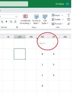
Only thing the cell M2 becomes quite Blurred and font changes to Segoe UI from Calibri which i normally use and Size from 11 changed to 8
Also the values drop down Vertically in the M Column from M2 onwards.

Same Effect as above when used your method with TOCOL

Will it be possible to have the values represented in ROW

Rapchik

 

[Fluff]

For horizontal use

=FILTER(SEQUENCE(,9),COUNTIFS(I2:K4,SEQUENCE(,9))=0)

The formula does not change the font, or font size.

 

[RapchikM]

=FILTER(SEQUENCE(9),COUNTIFS(I2:K4,SEQUENCE(9))=0)

Indeed Excellent.

The formula does not change the font, or font size

Pleas don't misunderstand me. It has changed. if you feel like you may forward these feedback to MS.
It has changed at cell where only formula has been written

Unable to upload image

Regards
RapchikM

 

[Fluff]

Typing a formula into a cell cannot change the format.

 

[RapchikM]

Sir Image is in front of you with red mark circle
Regds
RapchikM

 

[Fluff]

That image does not tell me anything. Are you just typing the formula, or copy/pasting from here?