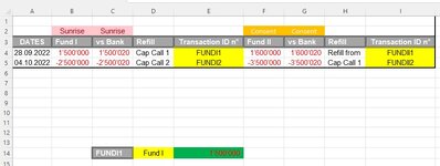
How to find a value based on 2 criteria: one horizontal and one vertical BUT which is not always in the same column.

[smetu]

Is there a way to find a formula in the green box based on the grey and yellow boxes.
The fact that the transaction ID's of Fund I and Fund II are not in the same columns prevents me to find a solution to this problem.....
It's been a head scratching for me for weeeeks!

 

[smetu]

can you give me the top-left most cell you're referencing and the bottom-right most cell??

A22 to TQ2752
(but the bottom-right will expand with time as I enter every day new transaction in this table and a few times a year I add also new funds)

 

[ExceLoki]

is this a named table/range?

 

[smetu]

Here's a screenshot of a piece of my table, to give you an idea if that can help.

 

[smetu]

is this a named table/range?

No it is not. I've tried with dynamic-naming the ranges (I mean to do dynamic named ranges), but if I add columns in the middle of my table then it shifts the ranges and the names don't fit the initial ranges anymore. It's a nightmare to find a solution to my problem.

 

[ExceLoki]

try this
you will need to edit
CELLWITHTEXTYOUARELOOKINGFOR1: dates, refill, vs bank, etc
CELLWITHTEXTYOUARELOOKINGFOR2: fundi1, fundii1, etc

=OFFSET(INDIRECT(ADDRESS(22,MATCH(CELLWITHTEXTYOUARELOOKINGFOR1,'[Private Equity Fund Dashboard.xlsx]DDowns & Distri'!$22:$22,0))),(MATCH(TRUE,MMULT(IFERROR(FIND(CELLWITHTEXTYOUARELOOKINGFOR2,FILTER('[Private Equity Fund Dashboard.xlsx]DDowns & Distri'!$A$22:$TQ$2752,'[Private Equity Fund Dashboard.xlsx]DDowns & Distri'!$A$22:$TQ$22="transaction id n*")),0),TRANSPOSE(SEQUENCE(1,COUNTIF('[Private Equity Fund Dashboard.xlsx]DDowns & Distri'!$22:$22,"transaction id n*"),1,0)))>0,0))-1,0)

 

[smetu]

try this
you will need to edit
CELLWITHTEXTYOUARELOOKINGFOR1: dates, refill, vs bank, etc
CELLWITHTEXTYOUARELOOKINGFOR2: fundi1, fundii1, etc

=OFFSET(INDIRECT(ADDRESS(22,MATCH(CELLWITHTEXTYOUARELOOKINGFOR1,'[Private Equity Fund Dashboard.xlsx]DDowns & Distri'!$22:$22,0))),(MATCH(TRUE,MMULT(IFERROR(FIND(CELLWITHTEXTYOUARELOOKINGFOR2,FILTER('[Private Equity Fund Dashboard.xlsx]DDowns & Distri'!$A$22:$TQ$2752,'[Private Equity Fund Dashboard.xlsx]DDowns & Distri'!$A$22:$TQ$22="transaction id n*")),0),TRANSPOSE(SEQUENCE(1,COUNTIF('[Private Equity Fund Dashboard.xlsx]DDowns & Distri'!$22:$22,"transaction id n*"),1,0)))>0,0))-1,0)

That's what I had done and it gives me "0".

 

[smetu]

That's what I had done and it gives me "0".

See?

 

[ExceLoki]

my initial guess, without being able to actually see either sheet entirely, would be that the search term "Transaction ID n*" does not show up the same number of times in both, or if there is anything else in row 22 of '[Private Equity Fund Dashboard.xlsx]DDowns & Distri'
'[Private Equity Fund Dashboard.xlsx]DDowns & Distri'!$A$22:$TQ$22
&
'[Private Equity Fund Dashboard.xlsx]DDowns & Distri'!$22:$22
this would make the mmult not return correctly

 

[smetu]

my initial guess, without being able to actually see either sheet entirely, would be that the search term "Transaction ID n*" does not show up the same number of times in both, or if there is anything else in row 22 of '[Private Equity Fund Dashboard.xlsx]DDowns & Distri'
'[Private Equity Fund Dashboard.xlsx]DDowns & Distri'!$A$22:$TQ$22
&
'[Private Equity Fund Dashboard.xlsx]DDowns & Distri'!$22:$22
this would make the mmult not return correctly

You are correct. In the Private Equity Fund Dashboard table (the source), there's all the funds (52 funds for now) and thus 52 times "Transaction ID" col.
Whereas in my result file, there's only one Fund, so only one Transaction ID col.

 

[ExceLoki]

that's not quite what i meant. if there are more or less cells with "Transaction ID" as the value in row 22 than there are in a22:tq22 then that will throw off the function.

try putting these in somewhere:

=FILTER('[Private Equity Fund Dashboard.xlsx]DDowns & Distri'!$A$22:$Q$25,'[Private Equity Fund Dashboard.xlsx]DDowns & Distri'!$A$22:$TQ$22="transaction id n*"))

&

=COUNTIF('[Private Equity Fund Dashboard.xlsx]DDowns & Distri'!$22:$22,"transaction id n*")

the number from the second one should match the number of columns returned by the first one