How do I get my formula to show blank when the data is actually blank, and zero when it's actually zero.

[AlenK37]

Hello. I'm relatively new to excel and been stuck on a formula now for a that I can't seem to figure out. For most of my data, I am using SUMIF's to get the information I need, which works good for about 99% of the data I need. However, it's leaving the zeros blank, but I need it actually show zeros as well when the result is zero. What is the best approach for this? Perhaps other formulas would be better? I'm currently extracting all the data into a table and referencing the data in my formulas.

Here is my current formula I am using: =IF(SUMIFS($D:$D,$A:$A,$AK127)="","",SUMIFS($D:$D,$A:$A,$AK127))

I've tried many variations of this code, but I still keep getting zero's for empty results.

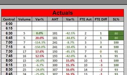
Side note, the data actually shows a "−" symbol when there is no data, not a blank

Any help or guidance would be much appreciated

 

[AlenK37]

Your screenshot didn't come through.
Are you saying in the formula bar you see a "-" ? How is the data getting there ?
I would have expected it to show either a formula or a 0.

I am copying data from one of my work systems via copy and paste. I have a table setup based off the data which is being pasted into A2:U97. The data I am looking at is time based, so depending on the time of the day, it will show a "-" if there is no data yet.

 

[Alex Blakenburg]

Assuming you only want to return "" if ALL the cells meeting the AK127 criteria are "-" then give this a try.

=IF(COUNTIFS($A:$A,$AK127,$D:$D,"-")=COUNTIFS($A:$A,$AK127),"",SUMIFS($D:$D,$A:$A,$AK127))

 

[AlenK37]

Assuming you only want to return "" if ALL the cells meeting the AK127 criteria are "-" then give this a try.

=IF(COUNTIFS($A:$A,$AK127,$D:$D,"-")=COUNTIFS($A:$A,$AK127),"",SUMIFS($D:$D,$A:$A,$AK127))

Yessss. This worked! Thank you!

 

[Alex Blakenburg]

You're welcome. Glad we could help.

 

[smozgur]

Yessss. This worked! Thank you!

The marked solution has been changed accordingly. In your future questions, please mark the post as the solution that actually answered your question, instead of your feedback message as it will help future readers. No further action is required for this thread.