Highlighting rows in a column when number changes (numbers are in consecutive order)

[mstaralynn]

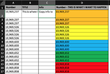
Hello - I have been trying to find a solution to this and have so far can up empty - but it seems like there HAS to be a way. I have a column with numbers in consecutive order - there could be 5 of one number, 3 of the next, 7 of the one after that - so I need to copy/paste info that correlates with the number. Problem is sometimes the numbers are similar and I miss the change and copy the wrong info. If I could have the rows colored, and change each Tim the number changes - I could visually see how far down I need to copy the info. The colors do not matter - its really just a visual guide. I tried the Conditional Formatting, Color Scales - and that doesn't work because they are in consecutive order. Also - find duplicates doesn't work either. Please see in the pic how I want the row to look - it could be the same 2 colors alternating at each number change - color doesn't matter. This is something I do very often and any way to make it easier is nice. THANK YOU!!!

 

[mstaralynn]

A couple of issues

1. You have applied Conditional Formatting to an entire column. How much data do you actually have? Since Conditional Formats are volatile I would not recommend applying them to an entire column as every time Excel recalculates for any reason the CF will have to evaluate all 2 x 1,048,576 CF formulas to determine if the cell should be formatted a particular way.
   
   
2. If you are going to apply the CF to cells below where the data is then a slight adjustment to the formula might be in order anyway.

So, in my dummy example below I have data in rows 2:12 but I want to allow for possible data down to row 20. I select from D2 (not D1) down to D20 and apply the shown CF formulas.
Is that something that you could adapt to suit your circumstances?

23 01 26.xlsm
	D
1	Number
2	a5
3	a5
4	a5
5	b3
6	b3
7	7
8	7
9	7
10	d6
11	e45
12	e45
13
14
15
16
17
18
19
20
Bands (2)

Cells with Conditional Formatting
Cell	Condition		Cell Format	Stop If True
D2:D20	Expression	=AND(ISEVEN(ROWS(UNIQUE(D$2:D2))),D2<>"")	text	NO
D2:D20	Expression	=AND(ISODD(ROWS(UNIQUE(D$2:D2))),D2<>"")	text	NO

Thank you!!!! This worked!! I didn't realize I needed to only select the data and not the entire column. There are around 450 rows. Thank you so much!

 

[Peter_SSs]

You're welcome. Thanks for the follow-up.