Got a headache trying to figure this one.

[dsims]

Ok so i did some data grabbing and I got one page that's full of data. I'm trying to pull data to one sheet based off two criteria. So if you use vlookup i can pull data based off one cell. In this case for example: (a1) apples (b2) red ..now based off my data grabbing there is a lot of apples and many different red but only row has apple then red on the same row ..by using these 2 as reference to pull the number of red apples...sry if this is confusing.

 

[Drrellik]

Welcome to the board,

if you could post some of your data it will help other understand what you are trying to do. as for Vlookup I think it likes your data to be sorted A-Z and then generally finds the first instance of the first condition like the first Apple and not the second one.

There is a link below to the XL2bb add on

 

[Peter_SSs]

Could you adapt something like this?

BTW, I suggest that you investigate XL2BB for providing sample data to make it easier for helpers by not having to manually type out sample data to test with.

23 08 08.xlsm
	A	B	C	D	E	F	G
1	Fruit	Colour	No.		Fruit	Colour	No.
2	apple	green	5		apple	red	10
3	apple	pink	3		apple	pink	3
4	pear	green	7		apple	green	5
5	pear	yellow	8		pear	yellow	8
6	apple	red	10		pear	green	7
7					banana	yellow	0
dsims

Cell Formulas
Range	Formula
G2:G7	G2	=SUMIFS(C$2:C$6,A$2:A$6,E2,B$2:B$6,F2)

 

[dsims]

Ok so i did some data grabbing and I got one page that's full of data. I'm trying to pull data to one sheet based off two criteria. So if you use vlookup i can pull data based off one cell. In this case for example: (a1) apples (b2) red ..now based off my data grabbing there is a lot of apples and many different red but only row has apple then red on the same row ..by using these 2 as reference to pull the number of red apples...sry if this is confusing.

Welcome to the board,

if you could post some of your data it will help other understand what you are trying to do. as for Vlookup I think it likes your data to be sorted A-Z and then generally finds the first instance of the first condition like the first Apple and not the second one.

There is a link below to the XL2bb add on

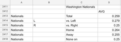
So the first pic is the a daily schedule of baseball. It automatically updates. I'm wanting to pull from page 2 the nationals avg for a R (right handed pitcher) so if i do a vlookup it only good for nationals but not for the nationals and R (right handed pitcher)

 

[Joe4]

Since you are using Excel 365, you should be able to use the new FILTER function.

So, if your other sheet really is named "Page 2", then place this formula in cell E2:

=FILTER('Page 2'!D:D,('Page 2'!A:A=Sheet3!A2)*('Page 2'!B:B=Sheet3!C2),"")

See here for more details on this FILTER function: FILTER function - Microsoft Support

 

[dsims]

Since you are using Excel 365, you should be able to use the new FILTER function.

So, if your other sheet really is named "Page 2", then place this formula in cell E2:

=FILTER('Page 2'!D:D,('Page 2'!A:A=Sheet3!A2)*('Page 2'!B:B=Sheet3!C2),"")

See here for more details on this FILTER function: FILTER function - Microsoft Support

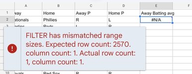
I'm pulling from page named "Splits" to page names "LHPRHP"

 

[Joe4]

So then just so what I said and replace "Page 2" with "Splits", i.e.

=FILTER(Splits!D:D,(Splits!A:A=Sheet3!A2)*(Splits!B:B=Sheet3!C2),"")

 

[dsims]

So then just so what I said and replace "Page 2" with "Splits", i.e.

=FILTER(Splits!D:D,(Splits!A:A=Sheet3!A2)*(Splits!B:B=Sheet3!C2),"")

So then just so what I said and replace "Page 2" with "Splits", i.e.

=FILTER(Splits!D:D,(Splits!A:A=Sheet3!A2)*(Splits!B:B=Sheet3!C2),"")

Got a n/a response.. this one is tricky

 

[Joe4]

Whoops, I forgot to remove the "Sheet3" reference.
Try this:

=FILTER(Splits!D:D,(Splits!A:A=A2)*(Splits!B:B=C2),"")

 

[dsims]

Whoops, I forgot to remove the "Sheet3" reference.
Try this:

=FILTER(Splits!D:D,(Splits!A:A=A2)*(Splits!B:B=C2),"")

Still getting a NA