Formula to calculate dinamically the average costs until the last non-blank cell

[vladimiratanasiu]

Hello!

I have a large table with monthly spendings. Some months they still don't happen, so that the correspondent cells are empty. I need a formula to calculate dinamically the average incurred costs until the last period with value, but counting also the previous months without spendings (see the results from column C).

Thank you!

Book1
	A	B	C
1	Month	Euro	Average
2	Jan-22	36.57	36.57
3	Feb-22	44.70	40.635
4	Mar-22
5	Apr-22	46.25	31.88
6	May-22	-7.12	24.08
7	Jun-22
8	Jul-22
9	Aug-22	33.32	19.215
10	Sep-22
11	Oct-22
12	Nov-22	14.36	15.28
13	Dec-22
14	Average
Sheet1

Cell Formulas
Range	Formula
C2	C2	=B2/1
C3	C3	=SUM(B2:B3)/2
C5	C5	=SUM(B2:B5)/4
C6	C6	=SUM(B2:B6)/5
C9	C9	=SUM(B2:B9)/8
C12	C12	=SUM(B2:B12)/11

 

[Fluff]

Ok, how about

=AVERAGE(--B2:INDEX(B1:B13,LOOKUP(99^99,B2:B13,ROW(B2:B13))))

 

[SanjayGMusafir]

Let me understand - You want average in Cell C14 from B2 to the cell in Column B that corresponds to the current month. Right or is it something different?

Is this what you needed - Check cell C14

All Records.xlsb
	A	B	C
1	Month	Euro	Average
2	Jan-2022	36.57	36.57
3	Feb-2022	44.70	40.64
4	Mar-2022
5	Apr-2022	46.25	31.88
6	May-2022	(7.12)	24.08
7	Jun-2022
8	Jul-2022
9	Aug-2022	33.32	19.22
10	Sep-2022
11	Oct-2022
12	Nov-2022	14.36	15.28
13	Dec-2022
14	Average	19.215
Sheet3

Cell Formulas
Range	Formula
C2	C2	=B2/1
C3	C3	=SUM(B2:B3)/2
C5	C5	=SUM(B2:B5)/4
C6	C6	=SUM(B2:B6)/5
C9	C9	=SUM(B2:B9)/8
C12	C12	=SUM(B2:B12)/11
B14	B14	=SUMIFS(B2:B13,A2:A13,"<="&TODAY())/COUNTIFS(A2:A13,"<="&TODAY())

 

[vladimiratanasiu]

What are you expecting for the result, 15.28, 14 or something else?

Ok, how about

=AVERAGE(--B2:INDEX(B1:B13,LOOKUP(99^99,B2:B13,ROW(B2:B13))))

Book1
	A	B	C
1	Month	Euro	Average
2	01/01/2022	36.57	36.57
3	01/02/2022	44.70	40.635
4	01/03/2022
5	01/04/2022	46.25	31.88
6	01/05/2022	-7.12	24.08
7	01/06/2022
8	01/07/2022
9	01/08/2022	33.32	19.215
10	01/09/2022
11	01/10/2022
12	01/11/2022	14.36	15.28
13	01/12/2022
14	Average	#VALUE!
Sheet1

Cell Formulas
Range	Formula
C2	C2	=B2/1
C3	C3	=SUM(B2:B3)/2
C5	C5	=SUM(B2:B5)/4
C6	C6	=SUM(B2:B6)/5
C9	C9	=SUM(B2:B9)/8
C12	C12	=SUM(B2:B12)/11
B14	B14	=AVERAGE(--B2:INDEX(B1:B13,LOOKUP(99^99,B2:B13,ROW(B2:B13))))

Am I missing any detail ? Is it possible on the B1 reference?

 

[Fluff]

Does column B contain formulae that return ""

 

[SanjayGMusafir]

Is this what you needed - Check cell C14

All Records.xlsb
	A	B	C
1	Month	Euro	Average
2	Jan-2022	36.57	36.57
3	Feb-2022	44.70	40.64
4	Mar-2022
5	Apr-2022	46.25	31.88
6	May-2022	(7.12)	24.08
7	Jun-2022
8	Jul-2022
9	Aug-2022	33.32	19.22
10	Sep-2022
11	Oct-2022
12	Nov-2022	14.36	15.28
13	Dec-2022
14	Average	19.215
Sheet3

Cell Formulas
Range	Formula
C2	C2	=B2/1
C3	C3	=SUM(B2:B3)/2
C5	C5	=SUM(B2:B5)/4
C6	C6	=SUM(B2:B6)/5
C9	C9	=SUM(B2:B9)/8
C12	C12	=SUM(B2:B12)/11
B14	B14	=SUMIFS(B2:B13,A2:A13,"<="&TODAY())/COUNTIFS(A2:A13,"<="&TODAY())

Did you check the above post vladimiratanasiu

 

[vladimiratanasiu]

Thank you very much, Fluff and SanjayGulatiMusafir! Both formulas run perfectly and I wish I could mark each one of them. However, giving the very large number of positive reviews accorded to Fluff, I decided to mark the SanjayGulatiMusafir solution. And hope it won't offend the other member.

 

[Fluff]

Both formulas run perfectly

I would disagree they both give totally different answers with your test data.

 

[vladimiratanasiu]

I would disagree they both give totally different answers with your test data.

Indeed, you are very right. After removing all values from both tables and inserting them again one by one, I noticed, to my shame, that the results are different. It was my mistake that I considered the two formulas available in any condition. Please excuse me, and if it's possible, change the marker from SanjayGulatiMusafir's solution to yours one. P.S. I'd appreciate if you could change the content from my previous message, keeping only the mention about your version.

 

[Fluff]

All you need to do is mark the post of your choice as the solution & it will override the one you have already marked.

 

[vladimiratanasiu]

All you need to do is mark the post of your choice as the solution & it will override the one you have already marked.

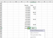
Thank you! One more question: I had to do some changes in my worksheet, meaning to move the respective table in other cells. As a result, the formula is no more working, giving the results from the attached image. The table references from the photo are the real cells, so that they can be used in the new solution.

Book2
	A	B	C
1
2
3		Month	Euro
4		1/1/2022	36.57
5		2/1/2022	44.7
6		3/1/2022
7		4/1/2022	46.25
8		5/1/2022	-7.12
9		6/1/2022
10		7/1/2022
11		8/1/2022	33.32
12		9/1/2022
13		########
14		########	14.36
15		########
16		Average	#REF!
Sheet1

Cell Formulas
Range	Formula
C16	C16	=AVERAGE(--C4:INDEX(C3:C15,LOOKUP(99^99,C4:C15,ROW(C4:C15))))