Excel formula needed

[FLdave12]

I have excel workbook with 4 sheets in it. It is a bid system workbook where employees bid by seniority for shift, days off and vacation time. The Master Sheet has members broken down by Shift Supervisors, Team Leads and Specialists. I have drop down menus with employee names, Choice of shifts (1st, 2nd, 3rd), and days off (SM, MT,TW, WT, TF, FR, and SS)

I have the other 3 sheets in the workbook labeled 1st, 2nd and 3rd. Each sheet has 6 months with rows for each month, day and date. I want members name and days off to auto fill based on the shift they selected. Also if possible approved vacation dates.
EX.
Month June 1 2 3 4 5 6 7 8 9 10 11 12 13 14
1st Shift S S M T W T F S S M T W T F
Employee 1 X X V V V

I am requesting assistance with formula or formulas to make this work. Appreciate any advice or assistance.



I would like an X to fill in for each employee days off. Ex. An X under day S & S for each of the 6 months.

 

[FLdave12]

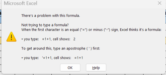
I apologize. I am doing something wrong. I am having trouble with entering the formulas.

I entered drop down menus for year and month in B1 and B2

On the 3rd shift sheet Cell A4 the month and year do not autopopulate.

Cell A5 does with 3rd shift based on the formula =TEXTAFTER(CELL("filename",A1),"]") & " shift"

Cell C5 when I entered formula =LET(mobegin,DATE(B1,MONTH(B2&1),1),SEQUENCE(1,DAY(EOMONTH(mobegin,0)),mobegin)) it gives the message #SPILL!

Same occurs when entered in C6 formula =CHOOSE(WEEKDAY(C5#),"S","M","T","W","T","F","S")

I had same issues with the other formulas.

Attached is screen shot with highlighted yellow areas not working.

Please advise and Thank you again

 

[KRice]

Let's take these one at a time:
1. Sounds like drop downs for year and month selections are okay in B1 and B2.
2. I don't believe my offering included a combined month and year in cell A4, but now that I look again, I think you want month-year in A5 and shift number in A6...is that correct (we can fix that easily)
The formula in Cell A5 would be moved to A6 if the answer to #2 is yes...and cell A5 would receive a different formula to display the month-year.
3. In cell C5, you're seeing the #SPILL error because the formula wants to automatically spill the results of a long array, but it needs empty cells to do so. Simply delete the contents of D5:AG5 and you'll see what the formula in C5 wants to deliver.
4. Same with cell C6...delete D6:AG6.
5. Not sure what you mean by "other formulas"...if they are #SPILL errors, delete any information in the original table that should be filled with new information.

 

[KRice]

Here is a minor revision that adds the Month-Year to A5 and moves the shift designation to A6. Note that A5 is formatted as a Date, to display as mmm-yy. If this is what you want, you can shorten the C5 formula a bit by replacing DATE(B1,MONTH(B2&1),1) with the cell reference (A5) since A5 effectively serves as a helper cell to describe the first day of the month of interest.

MrExcel_20231122.xlsx
	A	B	C	D	E
1	Year	2024
2	Month	March
3
4
5	Mar-24	Members	1	2	3
6	3rd Shift		F	S	S
7	Shift Supervisor	delta	X	V	V
8	Classification Specialist	golf
9	Classification Specialist	oscar
10
3rd

Cell Formulas
Range	Formula
C5:AG5	C5	=LET(mobegin,DATE(B1,MONTH(B2&1),1),SEQUENCE(1,DAY(EOMONTH(mobegin,0)),mobegin))
C6:AG6	C6	=CHOOSE(WEEKDAY(C5#),"S","M","T","W","T","F","S")
A5	A5	=DATE(B1,MONTH(B2&1),1)
A6	A6	=TEXTAFTER(CELL("filename",A1),"]") & " Shift"
A7:AG9	A7	=LET(sht,TEXTAFTER(CELL("filename",A1),"]"),ary,FILTER(tblMaster,tblMaster[Shift]=sht,""), pm,CHOOSECOLS(ary,1,2), v1st,CHOOSECOLS(ary,5),v2nd,CHOOSECOLS(ary,6), v1b,IFERROR(TEXTBEFORE(v1st,"-")+0,""),v1e,IFERROR(TEXTAFTER(v1st,"-")+0,""),v2b,IFERROR(TEXTBEFORE(v2nd,"-")+0,""),v2e,IFERROR(TEXTAFTER(v2nd,"-")+0,""), doi,MATCH(CHOOSECOLS(ary,4),{"SM","MT","TW","WT","TF","FS","SS"},0), vdo,IF(((C5#>=v1b)*(C5#<=v1e)+(C5#>=v2b)*(C5#<=v2e)>0),"V", IF(((MOD(doi-1,7)+1=WEEKDAY(C5#))+(MOD(doi,7)+1=WEEKDAY(C5#))>0),"X","")), HSTACK(pm,vdo))
Dynamic array formulas.

Cells with Data Validation
Cell	Allow	Criteria
B2	List	January,February,March,April,May,June,July,August,September,October,November,December

 

[KRice]

Just to clarify, the five cells in the last example (A5, A6, A7, C5, and C6) are the only cells into which formulas are entered. The last three of those cells mentioned will automatically spill their results.

 

[FLdave12]

Just to clarify, the five cells in the last example (A5, A6, A7, C5, and C6) are the only cells into which formulas are entered. The last three of those cells mentioned will automatically spill their results.

Still having some issues:
1. When I enter formula =LET(mobegin,DATE(B1,MONTH(B2&1),1),SEQUENCE(1,DAY(EOMONTH(mobegin,0)),mobegin)) it is giving result of 45292.0 then 45293 etc. Thought it was the format in cells but everything tried did not result in 1 2 3 for sequence of days of month
Also should rest of months Feb, March etc, autopopulate or do I need to enter formulas for each month?

2. Do I remove the Shift Supervisor, Team Lead and Specialists from column A rows 7, 8, and 10? Do they autopopulate from Master sheet?

Sorry again, just not that familiar with these types of excel formulas

Thank you

 

[FLdave12]

Still having some issues:
1. When I enter formula =LET(mobegin,DATE(B1,MONTH(B2&1),1),SEQUENCE(1,DAY(EOMONTH(mobegin,0)),mobegin)) it is giving result of 45292.0 then 45293 etc. Thought it was the format in cells but everything tried did not result in 1 2 3 for sequence of days of month
Also should rest of months Feb, March etc, autopopulate or do I need to enter formulas for each month?

2. Do I remove the Shift Supervisor, Team Lead and Specialists from column A rows 7, 8, and 10? I entered the formula in A7 and got message problem with formula.

Do they autopopulate from Master sheet?

Sorry again, just not that familiar with these types of excel formulas

Thank you


View attachment 102505

 

[KRice]

Have a look at the 2nd paragraph of post #10…

C5# (meaning cell C5 and the additional array elements that spill from it) are formatted as dates, and the display format is "d" to show only the day-of-the-month number.

Where you want 1,2,3,…, that array actually consists of dates, which Excel treats as numbers, specifically the number of days since a baseline “0” day reference point. So the sequential values you see in the 45 thousand range are correct. However, you’ll need to customize the display format for those 31 cells that might receive a date from the formula that spills, formatted such that only the day number is displayed. This is done by selecting those cells, then right click, Format Cells, then choose Custom and in the Type: field, enter d, then OK to exit. As an example, if the first cell is March 1, 2024, the actual behind-the-scenes value for that date on my system is 45352, but the customized display format shows 1 (because the date is day 1 of March).

You do not need any data in column A where the position, member, and days off results are to be displayed…other then the single formula in the upper left of the data table. The positions and members will spill down from that point.

Can you tell me more about the other months? These formulas will not create a multi-month output. What would that look like? If March 2024 is selected in B1:B2, do you want to see a table for March (currently done with approach shown above), a similar table below that for April, followed by tables for May, June, July, and August…always 6 months beginning with the initially selected month?

 

[FLdave12]

I will try all of your suggestions tomorrow and report back.

Do I put the A7 formula for positions in cell A7 or somewhere else?

Would it work if I put year and month columns over each month with formula to have month date and day autofill?

 

[KRice]

Regarding the A7 question, yes…a single formula in A7 is all that is needed. That formula creates the entire output table, although it does not split the output into separate sections with supervisors/team leaders appearing in an upper section followed by a blank row, and then followed by specialists. After trying it out, let me know if that works okay or if some other output format is desired.

Regarding the other question about month and year rows, those could be added, but they are not needed. The main results formula does not require such helper rows. The row discussed earlier (C5#) that shows that month’s day number actually contains a complete date, and that is used to determine whether each day falls on the member’s “weekend” or within a vacation block.

 

[FLdave12]

Regarding the A7 question, yes…a single formula in A7 is all that is needed. That formula creates the entire output table, although it does not split the output into separate sections with supervisors/team leaders appearing in an upper section followed by a blank row, and then followed by specialists. After trying it out, let me know if that works okay or if some other output format is desired.

Regarding the other question about month and year rows, those could be added, but they are not needed. The main results formula does not require such helper rows. The row discussed earlier (C5#) that shows that month’s day number actually contains a complete date, and that is used to determine whether each day falls on the member’s “weekend” or within a vacation block.

The A7 Cell with formula is still not working. Also, when I change the month it does not change the other months see attached: