Countif- Visible Cells in Filter mode

[aabbasi]

Hi:

Could someone please let me know the solution for the following problem:

I have values in cell B2:B50 with values such as Quality, Eng, Purchasing etc. When i go in Auto filter based on Coulmn A2:A50 (with July only) and count "Quality" manually under B2:B50, the answer is 26. But if I write formula Countif(B2:B50, "Quality") I get answer 41.

Is there a way to use Countif function, if I am in the Autofilter mode so as it counts only that rows which are visible under Autofilter and not ALL rows.

Thank you

 

[bmcmay]

Thank you so much ! Perfect

 

[Aladin Akyurek]

Thank you so much ! Perfect

You are welcome.

 

[denzo36]

Hi guys,

This problem is very interesting and I think I understand the solution for counting filtered data in a single column. I wonder can this solution be extended to counting data in multiple columns?

I have a data set that can be potentially be 13 columns wide and several thousand rows depending on the range of the date period I am looking at.

The data is a list of policy numbers and whether that policy had a 'referral code' associated with it or not. There are up to 100 different referral codes which are basically just different 5 digit numbers with each code having an explanation behind it (e.g. code 12345 means 'Driver with previous convictions' for example).

A policy can have either no referral code or potentially up to 13 referral codes depending on the situation. Each policy number is listed on one row with referral codes separated into different columns. Each of the 'referral' columns can contain any one of the 100 different referral rules. I can find the count of each referral code in the data set easily but would like the calculations to update when I change the filter on my date range. See image attached which should make more sense, I've simplified the data to 7 referral columns.

Would anyone have an idea how to tackle the added complication of multiple columns when the data is filtered?

For the unfiltered data I've listed all 100 referral codes in one column and used =COUNTIF(alldata,referral code) which works fine. I tried the below formula to extend the current formula given previously to include the columns in the offset function but that was more of an educated guess. This formula is based on the 'referral' 1 to 7 columns going from C to I and rows from C2 to C344. The last part of the formula $C$2:$I$344=B347 is comparing one of the referral codes which is in cell B347 to see if it is in the unfiltered range.

=SUMPRODUCT(SUBTOTAL(3,OFFSET($C$2:$C$344,ROW($C$2:$C$344)-MIN(ROW($C$2:$C$344)),COLUMN($C$1:$I$1)-1,1))*($C$2:$I$344=B347))

Any help would be appreciated.

 

[Vishal Revankar]

Thank you @Aladin Akyurek for your fantastic formula which would have helped thousands of people including me.

However, my current requirement is to achieve the same, provided my data is not limited to one column but is spread across multiple columns (very similar to what @denzo36 mentioned in his post above). @Aladin Akyurek would you be able to help me here please? Hope you are still active on this forum (fingers crossed)!

This is my sample table wherein I want to count working days (or leave days) for each team in a week/month/quarter.

			Jan	Jan	Jan	Jan	Jan	Jan	Jan
Emp ID	Name	Team	25	27	27	28	29	30	31
1110	Name 1	Team 1	W	W	W	W	W	S	S
1111	Name 2	Team 1	W	L	W	L	W	S	S
1112	Name 3	Team 2	W	W	W	W	W	S	S
1113	Name 4	Team 2	W	W	W	L	W	S	S
1114	Name 5	Team 2	L	L	W	W	W	S	S
1115	Name 6	Team 3	W	W	W	W	W	S	S
1116	Name 7	Team 3	W	W	L	W	W	S	S

 

[Fluff]

@Vishal Revankar
Please start a new thread for your question. Thanks

 

[Ramneek]

=SUMPRODUCT(SUBTOTAL(3,OFFSET(B2:B50,ROW(B2:B50)-MIN(ROW(B2:B50)),,1))*(B2:B50="Quality"))

Same problem faced today, searched Mr. Excel Message Board and as always Aladin's solution is there.

 

[Ramneek]

It's SUBTOTAL that is sensitive to visible cells. The function num 3 (i.e., COUNTA) yields 1 if any data in a given visible cell, otherwise 0 along with all non-visible cells.

Suppose we have it for a shorter range:

=SUMPRODUCT(SUBTOTAL(3,OFFSET(B2:B7,ROW(B2:B7)-MIN(ROW(B2:B7)),,1))*(B2:B7="Quality"))

Evaluationg just the row bit we get:

SUMPRODUCT(SUBTOTAL(3,OFFSET(B2:B7,{0;1;2;3;4;5},,1))*(B2:B7="Quality"))

SubTOTAL gets applied successively on

OFFSET(B2,0,,1)
OFFSET(B2,1,,1)
OFFSET(B2,2,,1)

and so on... leading to something like:

SUMPRODUCT({0;0;1;0;0;1}*(B2:B7="Quality"))

Cells with 1 do house data. If the data housed in the corresponding range is equal to "Quality", that cell is counting in.

Aladin Sahab, it is an awesome solution just like some mathematical derivation......Sir, I only would like to know one thing why you used B2:B7 in offset reference as when I applied your formula while only taking B2 in offset reference portion, it is still working. Would you be so kind to let me know the reason for the same.

Thanks

 

[Julie0511]

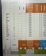
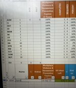
Hello, I have this worksheet which I used this amazing formula above, but I have an additional question.
When I filter between different groups the number stays the same all the way down? It’s there a way the numbers can reflect the groups you select in their specific row?