Copy column values from another sheet but want to exclude some specific row name completely..

pankajgrover

Board Regular
Joined
Oct 27, 2022
Messages
157
Office Version
  1. 2021
Platform
  1. Windows
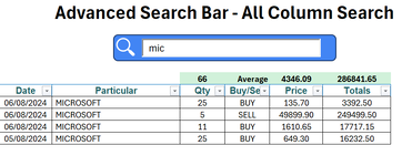
Copy column values from another sheet but want to exclude some specific row name completely . in example in B2 i want to exclude complete row name "Samsung" & "Netflix". how to do that ?

Cell Formulas
RangeFormula
A2:A17A2=IF(raw_data!A2="","",DATEVALUE(TEXT(raw_data!A2,"dd/mm/yyyy")))
B2:B17B2=IF(raw_data!C2="","",REPLACE(raw_data!C2,1,3,""))
C2:E17C2=IF(raw_data!D2="", "",raw_data!D2)
F2:F17F2=IFERROR([@Qty]*[@Price],"")
Named Ranges
NameRefers ToCells
all=raw_data!$A$2:$G$989A2
 
Good news. (y)


If you want the results in a formal table then there will need to be more formulas ..
(Check the table name in the formulas)

Cell Formulas
RangeFormula
A2:A18A2=IFERROR(INDEX(INT(FILTER(raw_data!A$2:A$200,raw_data!D$2:D$200<>"")),ROW()-ROW(Table1[#Headers])),"")
B2:B18B2=IFERROR(REPLACE(INDEX(FILTER(raw_data!C$2:C$200,raw_data!D$2:D$200<>""),ROW()-ROW(Table1[#Headers])),1,4,""),"")
C2:C18C2=IFERROR(INDEX(FILTER(raw_data!D$2:D$200,raw_data!D$2:D$200<>""),ROW()-ROW(Table1[#Headers])),"")
D2:D18D2=IFERROR(INDEX(FILTER(raw_data!E$2:E$200,raw_data!D$2:D$200<>""),ROW()-ROW(Table1[#Headers])),"")
E2:E18E2=IFERROR(INDEX(FILTER(raw_data!F$2:F$200,raw_data!D$2:D$200<>""),ROW()-ROW(Table1[#Headers])),"")
Perfect Working .. Yours previous and also this formula amazing.. So much Thank You :love: (y)
 
Upvote 0

Excel Facts

How to find 2nd largest value in a column?
MAX finds the largest value. =LARGE(A:A,2) will find the second largest. =SMALL(A:A,3) will find the third smallest
Good news. (y)


If you want the results in a formal table then there will need to be more formulas ..
(Check the table name in the formulas)

Cell Formulas
RangeFormula
A2:A18A2=IFERROR(INDEX(INT(FILTER(raw_data!A$2:A$200,raw_data!D$2:D$200<>"")),ROW()-ROW(Table1[#Headers])),"")
B2:B18B2=IFERROR(REPLACE(INDEX(FILTER(raw_data!C$2:C$200,raw_data!D$2:D$200<>""),ROW()-ROW(Table1[#Headers])),1,4,""),"")
C2:C18C2=IFERROR(INDEX(FILTER(raw_data!D$2:D$200,raw_data!D$2:D$200<>""),ROW()-ROW(Table1[#Headers])),"")
D2:D18D2=IFERROR(INDEX(FILTER(raw_data!E$2:E$200,raw_data!D$2:D$200<>""),ROW()-ROW(Table1[#Headers])),"")
E2:E18E2=IFERROR(INDEX(FILTER(raw_data!F$2:F$200,raw_data!D$2:D$200<>""),ROW()-ROW(Table1[#Headers])),"")
Sir, if i add search box in this sheet, and i want to search in Col B2 only, as i type ..is this possible.. search in any character in Col B2 and this way data will be filtered through search box.. thanks..
 
Upvote 0
here like this below example if i want to filter data through B column and A column.. so every time i did not need to go dropdown and tick and clear the filter...

Shares Search Filter APPLE.xlsx
ABCDEF
1Filter options:
2Stocks
3Date
4
source_data
 
Upvote 0
here like this below example if i want to filter data through B column and A column.. so every time i did not need to go dropdown and tick and clear the filter...
You shouldn't need a separate search box or to tick & clear filter
If you click on the clip below the list is originally filtered on Microsoft and I want to filter on Apple instead. When I click the filter drop-down and (not clearing anything) type an 'a' in the built-in search box you see anything with an 'a' appears in the list below. That is two items but as soon as I also type the 'p' that bottom list reduces to 'Apple' only and I simply press Enter to get the new filter.
 

Attachments

  • Filter.gif
    Filter.gif
    68.8 KB · Views: 4
Upvote 0
You shouldn't need a separate search box or to tick & clear filter
If you click on the clip below the list is originally filtered on Microsoft and I want to filter on Apple instead. When I click the filter drop-down and (not clearing anything) type an 'a' in the built-in search box you see anything with an 'a' appears in the list below. That is two items but as soon as I also type the 'p' that bottom list reduces to 'Apple' only and I simply press Enter to get the new filter.
Yeah that's a good idea. But just for learning purpose i want to know what will be formula in particular and date col. , i know how create search box and link with cell. But no knowledge about complex formula. I think it will be something like FILTER(my_data,NOT(ISERROR(SEARCH .... , but i did not know how to integrate with your given previous formula for particular Col. =IF(raw_data!C2="","",REPLACE(raw_data!C2,1,3,"")) and for Date col. =IF(raw_data!A2="","",DATEVALUE(TEXT(raw_data!A2,"dd/mm/yyyy"))) Thanks
 
Upvote 0
i want to search in Col B2 only, as i type .
If you want to search "as you type" then a formula will not do that. A formula will only update when you complete an entry in the input cell.
 
Upvote 0
If you want to search "as you type" then a formula will not do that. A formula will only update when you complete an entry in the input cell.
What i did now, i create new worksheet name search_bar and retrieve data from your previous formula sheet, i learn from youtube just now, and its working you can see if i type mic .. microsoft appears.. but here i also want another cell filter on date.. what will be formula in A8 if i filter on date also.. thanks
searchbox screenshot attached..

Shares Search Filter APPLE.xlsx
ABCDEF
1micAdvanced Search Bar - All Column Search
2
3
4
5
666Average4346.09286841.65
7DateParticularQtyBuy/SellPriceTotals
806/08/2024 MICROSOFT25BUY135.703392.50
906/08/2024 MICROSOFT5SELL49899.90249499.50
1006/08/2024 MICROSOFT11BUY1610.6517717.15
1105/08/2024 MICROSOFT25BUY649.3016232.50
search_bar
Cell Formulas
RangeFormula
C6,F6C6=SUBTOTAL(9,C8:C1000)
E6E6=F6/C6
A8:F11A8=FILTER(my_data,NOT(ISERROR(SEARCH(A1,my_data[Particular]))),"")
Dynamic array formulas.
Cells with Conditional Formatting
CellConditionCell FormatStop If True
A8:F1000Celldoes not contain a blank value textNO
 

Attachments

  • Screenshot 2024-08-13 170327.png
    Screenshot 2024-08-13 170327.png
    27 KB · Views: 1
Upvote 0
If you want to search "as you type" then a formula will not do that. A formula will only update when you complete an entry in the input cell.
hi @Peter_SSs how are you. you are right, formula will only work when complete an entry in the input cell and press enter. so with the help of you and others respected members, here below finally we reached our goal, but now issue arises it works on only 365 not work on 2021 excel. kindly you please look and alter formula that also work in 2021 excel. Thanks for always helping me... I think HSTACK function causes disruption in 2021 excel. Here is below formula for your reference..:

Excel Formula:
=FILTER(HSTACK((INT(Table1[Date])),REPLACE(Table1[Stocks],1,4,""),Table1[[Qty]:[Price]]),(NOT(ISERROR(SEARCH(B2,Table1[Stocks])&(SEARCH(C2,(INT(Table1[Date])))&(SEARCH(D2,Table1[Buy/Sell]))))))*(INT(Table1[Date])>=IF(E2="",1/1/1900,E2))*(INT(Table1[Date])<=IF(H2="",TODAY(),H2))*((Table1[Price])<=IF(I2="","",I2))*((Table1[Price])>=IF(J2="",1,J2))*(Table1[Qty]<>""))
 
Upvote 0
  1. Could we have a sample of Table1 data with XL2BB so we could have something realistic to test with?

  2. Can you explain in words what the formula is supposed to do?
 
Upvote 0

Forum statistics

Threads
1,221,310
Messages
6,159,176
Members
451,543
Latest member
cesymcox

We've detected that you are using an adblocker.

We have a great community of people providing Excel help here, but the hosting costs are enormous. You can help keep this site running by allowing ads on MrExcel.com.
Allow Ads at MrExcel

Which adblocker are you using?

Disable AdBlock

Follow these easy steps to disable AdBlock

1)Click on the icon in the browser’s toolbar.
2)Click on the icon in the browser’s toolbar.
2)Click on the "Pause on this site" option.
Go back

Disable AdBlock Plus

Follow these easy steps to disable AdBlock Plus

1)Click on the icon in the browser’s toolbar.
2)Click on the toggle to disable it for "mrexcel.com".
Go back

Disable uBlock Origin

Follow these easy steps to disable uBlock Origin

1)Click on the icon in the browser’s toolbar.
2)Click on the "Power" button.
3)Click on the "Refresh" button.
Go back

Disable uBlock

Follow these easy steps to disable uBlock

1)Click on the icon in the browser’s toolbar.
2)Click on the "Power" button.
3)Click on the "Refresh" button.
Go back
Back
Top