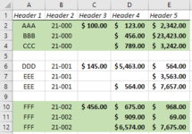
Conditional format groups of rows based on multiple criteria

[wiseone]

I have some data as listed in the below table with an example of how it would conditionally format.

It should format the rows based on the following criteria:

1. The group of items is highlighted based on column B* IF:
   • The first row of the group in cell column C is not blank.
   • The data in columns D and E for the group are not blank.
2. There is a blank row between groups, this should not highlighted.

*I would prefer it to group just based on Columns C D and E, and recognized they are separated by blank rows, but I don't think this is possible...so I instead suggested column B as a means to group them....if you think you can suggest a way to ignore column B....I'd love to see your suggestion.

Thanks in advance for your help!

 

[Eric W]

Are you specifically having performance issues? The COUNTIF and COUNTIFS functions are "aware" of the last row used, so if you only have 500 lines, that's all it looks at. If you've done something odd, like having a few thousand lines at the end, then deleted those lines, then Excel might not know the "real" end until you save the workbook again. So that leaves the MATCH function. I did not specifically test the formula on a large range, but I thought that since the MATCH would definitely find a match (except for blank rows) within the actual range, it should go quickly. But if you are having performance issues, or you just want to switch to a specific range, you can do it. You're very close in fact:

=AND(INDEX($AI$6:$AI$500,MATCH($R6,$R$6:$R$500,0))<>"",COUNTIF($R$6:$R$500,$R6)*3=COUNTIFS($R$6:$R$500,$R6,$AC$6:$AC$500,"<>")+COUNTIFS($R$6:$R$500,$R6,$AD$6:$AD$500,"<>")+ COUNTIFS($R$6:$R$500,$R6,$AK$6:$AK$500,"<>"))

You just needed to make the ranges absolute. I also realized that the $A6<>"" condition wasn't necessary (at least on my sample sheet).

 

[wiseone]

Thanks, I'll test it out again, delete anything that might be hidden and save and see if it works without performance problems. Appreciate it.

 

[wiseone]

Hi @Eric W , Hoping you can help with this one again. Been a long while and I am still using your suggestion in my spreadsheet. Over time, it grows from 10 rows to ~530 rows. My sheet resets every year, so towards mid-year I start to notice a slow down in the response time of the sheet when I am typing in cells. Can you think of any way to make this formula less demanding?

The Criteria:

For Groups Rows of Data separated by blank rows....

The conditional format should highlight all rows which meet these conditions and are matched by the code in Column R.

• Everything in Column A must not be Blank
• Everything in Column R must Match
• Everything in Column AD must not be blank
• Everything in Column AK must not be blank
• The top row of AP must not be blank.
• Everything in Column AR must not be blank

Here is the formula as it is today....working, but gets slow as the table grows....

=AND($A6<>"",INDEX($AP$6:$AP$536,MATCH($R6,$R$6:$R$536,0))<>"",COUNTIF($R$6:$R$536,$R6)*3=COUNTIFS($R$6:$R$536,$R6,$AD$6:$AD$536,"<>")+COUNTIFS($R$6:$R$536,$R6,$AK$6:$AK$536,"<>")+ COUNTIFS($R$6:$R$536,$R6,$AR$6:$AR$536,"<>"))

Thanks!

 

[Eric W]

I've played around with this a bit. I've had a bit of a tough time working on this, since I didn't notice any slowdown with any of the formulas I tested, even with over 1000 lines and all 3 formulas running at the same time. Also, please update your profile to show what version of Excel you're using, it can make a difference in what functions that are available for you to use. That said, consider this:

Book1
	A																	R												AD							AK					AP		AR	AS	AT	AU
1
2
3
4	Header 1																	Header 2												Header 4							Header 5					Header 3		Header 6
5
6	AAA																	21-000												123							2342					100		1	TRUE	TRUE	TRUE
7	BBB																	21-000												456							23423							2	TRUE	TRUE	TRUE
8	CCC																	21-000												789							3242							3	TRUE	TRUE	TRUE
9																																													#N/A	#N/A	FALSE
10	DDD																	21-001												5463							564					15		4	FALSE	FALSE	FALSE
11	EEE																	21-001																			3563							5	FALSE	FALSE	FALSE
12	EEE																	21-001												564							7657							6	FALSE	FALSE	FALSE
13																																													#N/A	#N/A	FALSE
14	FFF																	21-002												675							968					456		7	TRUE	TRUE	TRUE
15	FFF																	21-002												909							69							8	TRUE	TRUE	TRUE
16	FFF																	21-002												6574							7675							9	TRUE	TRUE	TRUE
17																																													#N/A	#N/A	FALSE
18	GGG																	21-003												5463							564							10	FALSE	FALSE	FALSE
19	HHH																	21-003												89							3563							11	FALSE	FALSE	FALSE
20	HHH																	21-003												564							7657							12	FALSE	FALSE	FALSE
21																																													#N/A	#N/A	FALSE
22	JJJ																	21-004																										1	FALSE	FALSE	FALSE
23	JJJ																	21-004																										2	FALSE	FALSE	FALSE
24	KKK																	21-004																								123		3	FALSE	FALSE	FALSE
25	KKK																	21-004																										4	FALSE	FALSE	FALSE
26																																													#N/A	#N/A	FALSE
27	LLL																	21-005																								456			FALSE	FALSE	FALSE
28	MMM																	21-005																								789			FALSE	FALSE	FALSE
29																																													#N/A	#N/A	FALSE
30	NN																	21-006												1							A					111		2	TRUE	TRUE	TRUE
31	OO																	21-006												2							B							3	TRUE	TRUE	TRUE
32	PP																	21-006												3							C							5	TRUE	TRUE	TRUE
33	QQ																	21-006												4							D							7	TRUE	TRUE	TRUE
34	RR																	21-006												5							E							11	TRUE	TRUE	TRUE
35	SS																	21-006												6							F							13	TRUE	TRUE	TRUE
36																																															FALSE
Sheet1 (2)

Cell Formulas
Range	Formula
AS6:AS35	AS6	=AND($A6<>"",INDEX($AP$6:$AP$536,MATCH($R6,$R$6:$R$536,0))<>"",COUNTIF($R$6:$R$536,$R6)*3=COUNTIFS($R$6:$R$536,$R6,$AD$6:$AD$536,"<>")+COUNTIFS($R$6:$R$536,$R6,$AK$6:$AK$536,"<>")+ COUNTIFS($R$6:$R$536,$R6,$AR$6:$AR$536,"<>"))
AT6:AT35	AT6	=LET(mr,10,rng,OFFSET($A6,MAX(-mr,1-ROW($R6)),0,mr*2,44),AND(VLOOKUP($R6,OFFSET(rng,0,17),25,0)<>"",SUM(COUNTIFS(OFFSET(rng,0,17,,1),$R6,OFFSET(rng,0,cols-1,,1),""))=0))
AU6:AU36	AU6	=IF(A6<>"",IF(A5="",AND(AP6<>"",SUM(COUNTIFS(R6:R16,R6,OFFSET(A6:A16,0,{1,30,37,44}-1),""))=0),AU5))

Cells with Conditional Formatting
Cell	Condition		Cell Format	Stop If True
AW:AW,AY:AY,AS:AU	Expression	=AS1	text	NO
A6:AR35	Expression	=LET(mr,10,rng,OFFSET($A6,MAX(-mr,1-ROW($R6)),0,mr*2,44),AND(VLOOKUP($R6,OFFSET(rng,0,17),25,0)<>"",SUM(COUNTIFS(OFFSET(rng,0,17,,1),$R6,OFFSET(rng,0,cols-1,,1),""))=0))	text	NO

Your current formula is in column AS, and it works fine. I came up with a shorter formula which is in column AT. You can see that I used it in the Conditional Formatting. It works too, but I can't really tell if it's more efficient or not. It also has some downsides. It requires Excel 365, it has a lot of "magic numbers" in it, and requires a Named constant (cols = {1,30,37,44}). In programming parlance, magic numbers are numbers in the code that have no explanation and seem like they just appear like magic. If you want to use this formula, I'll explain where these values came from, mostly column numbers, or differences between column numbers. For example, cols contains the column numbers of the columns that have to have all rows filled (A, AD, AK, AR). The main reason I thought that it might be more efficient is that it only checks 10 rows for each group. The mr at the start stands for max-rows, and you can change that as desired. I don't know how many rows a section could have.

Another thought I had is to just use a helper column. If you put your formula in AS6 and drag down, then you can change your CF formula to =$AS6. So the complicated formula only has to calculate once per row, which should speed things up. Same thing with the AT formula if you want to use that. Then I considered that if you do use a helper column, the formula could be simplified even more, giving rise to the AU formula. Again, this only checks 10 rows maximum, but this is incorporated in the A6:A16 range, change to A6:A26 or whatever makes sense.

Anyway, hope you find something useful in this!