Complicated formula

[Bartjeuh78]

Hi there all.
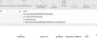
I have a question for the experts here. I hope I can upload the example sheet to make it more clear. I hope it works when openend in an English version of excel. My version is Dutch with Office 365. The yellow data set D4 to R12 is a working formula. I did not made this formula, it is way too complex for me to understand this formula. But now I want this formula somewhat modified. I need 3 extra columns to add to the formula. How it should look is in cells D16 to U24. The yellow is the original formula data, the green is what needs to be added. The working formula gets the data from every month-sheet January to December from cells L6 to M15. The more detailled formula must get the info from cells D6 to H15. The data is exactly the same, just 3 more columns. Who can build this formula? I want it in a formula like the first data set, not a pivot table, and no power query.
Who can help me with this? Thx in advance.
Bart

Laatste Update Budgetfile Ingekort.xlsx
	D	E	F	G	H	I	J	K	L	M	N	O	P	Q	R	S	T	U
2	This is the working forumula for dataset L6 to M15
3	Name	January	February	March	April	May	June	July	August	September	Oktober	November	December	Tot. Year	Avg / Month
4	Autoverzekering				$ 400.00									$ 400.00	$ 400.00
5	Fitness	$ 50.00	$ 50.00	$ 50.00	$ 50.00									$ 200.00	$ 50.00
6	GSM	$ 30.00	$ 30.00	$ 30.00	$ 30.00									$ 120.00	$ 30.00
7	Inboedelverzekering	$ 400.00												$ 400.00	$ 400.00
8	Lidgeld postzegel club	$ 25.00												$ 25.00	$ 25.00
9	Modelbouwclub		$ 40.00											$ 40.00	$ 40.00
10	Netflix			$ 25.00	$ 25.00									$ 50.00	$ 25.00
11	Spotify			$ 20.00	$ 20.00									$ 40.00	$ 20.00
12	TV	$ 40.00	$ 40.00	$ 40.00	$ 40.00									$ 160.00	$ 40.00
13
14	Now I need a formula where 3 extra colums are added. The dataset is D6 to H15 for every month. Fist sorted on column D, then column E
15	Sort	Name	Periodicidy	Info field	January	February	March	April	May	June	July	August	September	Oktober	November	December	Tot. Year	Avg / Month
16	ABONNEMENT	Fitness	MAANDELIJKS		$ 50.00	$ 50.00	$ 50.00	$ 50.00									$ 200.00	$ 50.00
17	ABONNEMENT	GSM	MAANDELIJKS		$ 30.00	$ 30.00	$ 30.00	$ 30.00									$ 120.00	$ 30.00
18	ABONNEMENT	Netflix	MAANDELIJKS				$ 25.00	$ 25.00									$ 50.00	$ 25.00
19	ABONNEMENT	Spotify	MAANDELIJKS				$ 20.00	$ 20.00									$ 40.00	$ 20.00
20	ABONNEMENT	TV	MAANDELIJKS		$ 40.00	$ 40.00	$ 40.00	$ 40.00									$ 160.00	$ 40.00
21	LIDGELD	Lidgeld postzegel club	JAARLIJKS		$ 25.00												$ 25.00	$ 25.00
22	LIDGELD	Modelbouwclub	JAARLIJKS			$ 40.00											$ 40.00	$ 40.00
23	VERZEKERING	Autoverzekering	JAARLIJKS	Polis nr 4321				$ 400.00									$ 400.00	$ 400.00
24	VERZEKERING	Inboedelverzekering	JAARLIJKS	Polis nr 12345	$ 400.00												$ 400.00	$ 400.00
25
Year Totals

Cell Formulas
Range	Formula
D4:R12	D4	=IFERROR(LET(x,VSTACK(January:DECEMBER!L6:M15),y,FILTER(x,(INDEX(x,,1)<>"")*(INDEX(x,,1)<>"selecteer")),u,UNIQUE(INDEX(y,,1)),jan,INDEX(January!M6:M15,MATCH(u,January!L6:L15,0)),feb,INDEX(February!M6:M15,MATCH(u,February!L6:L15,0)),mrt,INDEX(March!M6:M15,MATCH(u,March!L6:L15,0)),apr,INDEX(APRIL!M6:M15,MATCH(u,APRIL!L6:L15,0)),mei,INDEX(May!M6:M15,MATCH(u,May!L6:L15,0)),jun,INDEX(June!M6:M15,MATCH(u,June!L6:L15,0)),jul,INDEX(July!M6:M15,MATCH(u,July!L6:L15,0)),aug,INDEX(August!M6:M15,MATCH(u,August!L6:L15,0)),sep,INDEX(SEPTEMBER!M6:M15,MATCH(u,SEPTEMBER!L6:L15,0)),okt,INDEX(October!M6:M15,MATCH(u,October!L6:L15,0)),nov,INDEX(NOVEMBER!M6:M15,MATCH(u,NOVEMBER!L6:L15,0)),dec,INDEX(DECEMBER!M6:M15,MATCH(u,DECEMBER!L6:L15,0)),z,INDEX(y,,2),s,MMULT(--(TOROW(INDEX(y,,1))=u),INDEX(y,,2)),r,SORT(HSTACK(u,jan,feb,mrt,apr,mei,jun,jul,aug,sep,okt,nov,dec,s),1),HSTACK(r,INDEX(r,,14)/INDEX(GROUPBY(y,y,COUNTA,0,0),,3))),"")
Dynamic array formulas.

 

[Joe4]

Barthjeuh78,

It looks like you had marked post 6 (your own post) as the solution, even though your question has not been solved.
I have unmarked it. Please do not mark a post as the solution if it does not solve your question.
If you get a reply that answers your question (or you figure it out yourself), you can then mark that post (if it contains the solution) as the solution.

Thank you,
The Moderators

 

[djclements]

Sounds good. Thanks @Rijnsent for the translation. Incidentally, I too had issues with Excel crashing when trying to highlight the entire formula (to copy and paste it here). I thought maybe it was just a one-off, but since you also experienced the same behavior, I suspect it's a glitch caused by Excel trying to evaluate the formula in the formula bar. If you copy it in smaller portions (e.g. the top half of the formula first, then the bottom half), it doesn't cause an app crash, presumably because Excel doesn't evaluate a highlighted section if it contains an incomplete formula. I'm guessing the crash in this particular case is due to a combination of the 3D range reference and one of the functions used (possibly PIVOTBY and/or GROUPBY, or maybe even the SHEETS function), but I haven't done any extensive testing as of yet to try to narrow it down.

Upon further testing, it seems the auto-evaluate bug was caused by defining the rng variable separately. If we move the 3D range reference inside of both VSTACK and SHEETS, Excel does not crash when highlighting the entire formula in the formula bar:

=LET(
    arr, VSTACK(JANUARI:DECEMBER!D6:H15),
    n, SHEETS(JANUARI:DECEMBER!D6:H15),
    ...
)

You could also define the 3D range reference in Name Manager; or, if the number of sheets is always the same, you could also just replace SHEETS(JANUARI:DECEMBER!D6:H15) with 12.

The more you know...

 

[Bartjeuh78]

Thx a lot guys, this really is what I needed. I would not be able to find this myself. One small question. As I tried the last solution from djclements, I got the mistake: The first argument of LET needs to be a valid name. Even when I translated it to Dutch, my excel language, I get the same error. So I guess there is something wrong with the last solution. Also, what I want to ask, for myself to understand the formula, why is there a (h*29) in the formula? H is a variable in the formula, but where comes the *29 from? Why is that needed?
Thx in advance.

 

[djclements]

Thx a lot guys, this really is what I needed. I would not be able to find this myself. One small question. As I tried the last solution from djclements, I got the mistake: The first argument of LET needs to be a valid name. Even when I translated it to Dutch, my excel language, I get the same error. So I guess there is something wrong with the last solution. Also, what I want to ask, for myself to understand the formula, why is there a (h*29) in the formula? H is a variable in the formula, but where comes the *29 from? Why is that needed?
Thx in advance.

"The first argument of LET needs to be a valid name" error can be caused if you didn't used the correct system separator (e.g. commas instead of semi-colons). I believe the following should work for you (assuming the translations are correct):

=LET(
    arr; VERT.STAPELEN(JANUARI:DECEMBER!D6:H15);
    n; BLADEN(JANUARI:DECEMBER!D6:H15);
    c; NAAR.KOLOM(ALS(REEKS(;RIJEN(arr)/n);REEKS(n)));
    r; KIES.KOLOMMEN(arr;1;2;3;5)&"";
    v; KIES.KOLOMMEN(arr;4);
    i; (NEMEN(arr;;1)<>"SELECTEER")*(NEMEN(arr;;1)<>"");
    p; DRAAIEN.PER(r;c;v;SOM;;0;;1;;i);
    h; DRUPPEL(NEMEN(p;1);;4);
    a; DRUPPEL(p;1);
    VERT.STAPELEN(
        HOR.STAPELEN("Soort";"Naam";"Periodiciteit";"Nota";TEKST(ALS.FOUT(h*29;"Totaal Jaar");"mmmm");"Gemiddelde / Maand");
        HOR.STAPELEN(a;NEMEN(a;;-1)/NEMEN(GROEPEREN.PER(r;v;RIJEN;;0;;i);;-1))
    )
)

Regarding the "h*29" portion of the formula, this is just a little trick to convert the numbers 1-12 to "January"-"December". h is the header row of the PIVOTBY results (p), which returns {1,2,3,4,"Total"} in your sample file (representing JANUARI thru APRIL, because they are the only worksheets containing data). {1,2,3,4,"Total"}*29 returns {29,58,87,116,#VALUE!}, which are interpreted in Excel as the dates 29-Jan-1900, 27-Feb-1900, 27-Mar-1900 and 25-Apr-1900. IFERROR replaces #VALUE! with "Totaal Jaar", and the TEXT function is used to format the dates as "mmmm". Note: I'm not sure if "mmmm" is the correct syntax for the TEKST function to return long month format in Dutch. Please adjust, if necessary.

 

[Bartjeuh78]

Hi there djclements,
Thx for the follow up. Now it worked fine. But the headers were not needed in the formula. Second remark: every empty month is not listed in the output of the formula. So the best formula this far is the solution I marked as the solution on page 1 of this thread. Thank you for the solution. This helped me a lot. I updated the example file, so the dropbox link should now link to the example file with the solution. I got what I needed.
Regards,
Bart

 

[Bartjeuh78]

I implemented the formula in the "real" file, and I found one annoying thing. The data is well captured, but the first line is a 0 over almost the first line. The actual data comes on the second line and further. Does anyone know how this comes? How to fix this? I uploaded a print screen. If needed I upload something via dropbox. But the forum says you need to anonymize data. In the test file it is showed perfectly, but in the real file there is a line with almost all "0" to start.

 

[Bartjeuh78]

No need to worry, I was panicking too fast. It was the cell formatting from the source file that was not correct. Now all is showing ok.