Can I please have an amendment to this conditional formatting

les361800

New Member
Joined
Jul 11, 2023
Messages
28
Office Version
  1. 365
Platform
  1. Windows
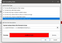
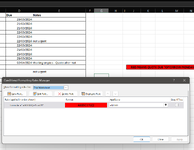
I was kindly provided with this formula to turn a cell red when the date was the next day.
The cell however turns back to white when the date is the current date - can it be amended so that it turns red the day before, and stays red when on or past the date?

Thank you :)
 

Attachments

  • Screenshot 2024-03-20 120635.png
    Screenshot 2024-03-20 120635.png
    33.9 KB · Views: 11
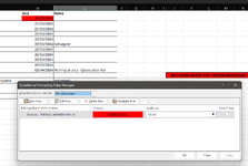
what is the conditional formatting rule that you have in cell
D2?

Does this help:

Book1
ABCDEF
119.03.2024TRUE
218.03.2024TRUE
317.03.2024TRUE
417.03.2024TRUE
518.03.2024TRUE
622.03.2024FALSE
717.03.2024TRUE
822.03.2024FALSE
922.03.2024FALSE
1022.03.2024FALSE
1122.03.2024FALSE
1218.03.2024TRUE
1318.03.2024TRUE
1418.03.2024TRUE
1522.03.2024FALSE
Sheet4
Cell Formulas
RangeFormula
F1:F15F1=TODAY()>WORKDAY(D1,-1)
Cells with Conditional Formatting
CellConditionCell FormatStop If True
D1:D15Expression=TODAY()>WORKDAY(D1,-1)textNO
 
Upvote 0

Excel Facts

Excel Joke
Why can't spreadsheets drive cars? They crash too often!
what is the conditional formatting rule that you have in cell
D2?

Does this help:

Book1
ABCDEF
119.03.2024TRUE
218.03.2024TRUE
317.03.2024TRUE
417.03.2024TRUE
518.03.2024TRUE
622.03.2024FALSE
717.03.2024TRUE
822.03.2024FALSE
922.03.2024FALSE
1022.03.2024FALSE
1122.03.2024FALSE
1218.03.2024TRUE
1318.03.2024TRUE
1418.03.2024TRUE
1522.03.2024FALSE
Sheet4
Cell Formulas
RangeFormula
F1:F15F1=TODAY()>WORKDAY(D1,-1)
Cells with Conditional Formatting
CellConditionCell FormatStop If True
D1:D15Expression=TODAY()>WORKDAY(D1,-1)textNO
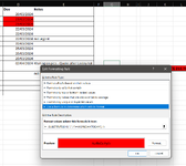
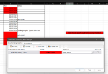
Hmm that doesnt appear to work.
Please see attached picture of your new formula and the one I currently have

Thank you so much for your help!
 

Attachments

  • Screenshot 2024-03-20 143225.png
    Screenshot 2024-03-20 143225.png
    68.2 KB · Views: 6
  • Screenshot 2024-03-20 143308.png
    Screenshot 2024-03-20 143308.png
    73.1 KB · Views: 5
Upvote 0
sorry, i had variables backwards:

Book1
ABCDEF
119.3.2024FALSE
218.3.2024FALSE
317.3.2024FALSE
417.3.2024FALSE
518.3.2024FALSE
622.3.2024TRUE
717.3.2024FALSE
822.3.2024TRUE
922.3.2024TRUE
1022.3.2024TRUE
1122.3.2024TRUE
1218.3.2024FALSE
1318.3.2024FALSE
1418.3.2024FALSE
1522.3.2024TRUE
Sheet1
Cell Formulas
RangeFormula
F1:F15F1=D1>WORKDAY(TODAY(),-1)
Cells with Conditional Formatting
CellConditionCell FormatStop If True
D1:D15Expression=D1>WORKDAY(TODAY(),-1)textNO
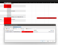
lol nope!
I might just manually change the dates... haha
 

Attachments

  • Screenshot 2024-03-20 144142.png
    Screenshot 2024-03-20 144142.png
    73.7 KB · Views: 7
Upvote 0
no, don't give up so easily.

Try:

Book1
ABCDEF
117.3.2024TRUE
218.3.2024TRUE
319.3.2024TRUE
420.3.2024TRUE
521.3.2024TRUE
622.3.2024FALSE
723.3.2024FALSE
824.3.2024FALSE
925.3.2024FALSE
1026.3.2024FALSE
1127.3.2024FALSE
1228.3.2024FALSE
1329.3.2024FALSE
1430.3.2024FALSE
1531.3.2024FALSE
Sheet1
Cell Formulas
RangeFormula
F1:F15F1=TODAY()+1>=D1
Cells with Conditional Formatting
CellConditionCell FormatStop If True
D1:D15Expression=TODAY()+1>=D1textNO
I commend your dedication!

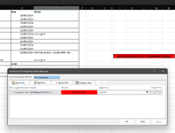
It still does nothing though! :(

I see you have something in F? I'm only trying to get the dates themselves to turn red, just the D column... dunno if that makes a difference?
 

Attachments

  • Screenshot 2024-03-20 145028.png
    Screenshot 2024-03-20 145028.png
    64.7 KB · Views: 6
Upvote 0
Why are you putting your conditional formula in QUOTES?

Column F is building a conditional formula to use for condition in column D.
If the formula in column give you the trues and falses you want, then that is the conditional formula to use.

Why don't you past a TABLE (Copy and Paste) a column D sample, an in column F tell me if it should be red or not.
Ahh I'm sorry, I was just copy and pasting! No idea why it was putting those in.

It looks like it works! It does make all the blank cells red too though... but I can live with it!
 

Attachments

  • Screenshot 2024-03-20 150036.png
    Screenshot 2024-03-20 150036.png
    66.5 KB · Views: 4
Upvote 0
It looks like it works! It does make all the blank cells red too though... but I can live with it!
It also won't highlight a Monday if you're looking at this on a Friday.

You may like this better;

Book1
ABCDEF
1Sun 17.3.2024TRUE
2Mon 18.3.2024TRUE
3Tue 19.3.2024TRUE
4Wed 20.3.2024TRUE
5Thu 21.3.2024TRUE
6Fri 22.3.2024FALSE
7Sat 23.3.2024FALSE
8Sun 24.3.2024FALSE
9Mon 25.3.2024FALSE
10Tue 26.3.2024FALSE
11Wed 27.3.2024FALSE
12Thu 28.3.2024FALSE
13Fri 29.3.2024FALSE
14Sat 30.3.2024FALSE
15Sun 31.3.2024FALSE
16FALSE
17FALSE
18FALSE
19FALSE
20FALSE
21FALSE
22FALSE
Sheet1
Cell Formulas
RangeFormula
F1:F22F1=AND(D1<>"",WORKDAY(TODAY(),1)>=D1)
Cells with Conditional Formatting
CellConditionCell FormatStop If True
D1:D15Expression=AND(D1<>"",WORKDAY(TODAY(),1)>=D1)textNO
 
Upvote 0
It also won't highlight a Monday if you're looking at this on a Friday.

You may like this better;

Book1
ABCDEF
1Sun 17.3.2024TRUE
2Mon 18.3.2024TRUE
3Tue 19.3.2024TRUE
4Wed 20.3.2024TRUE
5Thu 21.3.2024TRUE
6Fri 22.3.2024FALSE
7Sat 23.3.2024FALSE
8Sun 24.3.2024FALSE
9Mon 25.3.2024FALSE
10Tue 26.3.2024FALSE
11Wed 27.3.2024FALSE
12Thu 28.3.2024FALSE
13Fri 29.3.2024FALSE
14Sat 30.3.2024FALSE
15Sun 31.3.2024FALSE
16FALSE
17FALSE
18FALSE
19FALSE
20FALSE
21FALSE
22FALSE
Sheet1
Cell Formulas
RangeFormula
F1:F22F1=AND(D1<>"",WORKDAY(TODAY(),1)>=D1)
Cells with Conditional Formatting
CellConditionCell FormatStop If True
D1:D15Expression=AND(D1<>"",WORKDAY(TODAY(),1)>=D1)textNO
Cool ,thanks!!

Hmm how come your empty boxes arent red too?
 

Attachments

  • Screenshot 2024-03-20 150629.png
    Screenshot 2024-03-20 150629.png
    75.9 KB · Views: 5
Upvote 0

Forum statistics

Threads
1,224,798
Messages
6,181,038
Members
453,014
Latest member
Chris258

We've detected that you are using an adblocker.

We have a great community of people providing Excel help here, but the hosting costs are enormous. You can help keep this site running by allowing ads on MrExcel.com.
Allow Ads at MrExcel

Which adblocker are you using?

Disable AdBlock

Follow these easy steps to disable AdBlock

1)Click on the icon in the browser’s toolbar.
2)Click on the icon in the browser’s toolbar.
2)Click on the "Pause on this site" option.
Go back

Disable AdBlock Plus

Follow these easy steps to disable AdBlock Plus

1)Click on the icon in the browser’s toolbar.
2)Click on the toggle to disable it for "mrexcel.com".
Go back

Disable uBlock Origin

Follow these easy steps to disable uBlock Origin

1)Click on the icon in the browser’s toolbar.
2)Click on the "Power" button.
3)Click on the "Refresh" button.
Go back

Disable uBlock

Follow these easy steps to disable uBlock

1)Click on the icon in the browser’s toolbar.
2)Click on the "Power" button.
3)Click on the "Refresh" button.
Go back
Back
Top