Calculate Lead Time - Critical Path.

[Morpheus2022]

Hi,

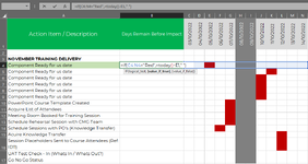
So I have a spreadsheet with list of training related project actions / tasks that need to be completed by a certain date. I need to calculate the date based on a colour in a cell.

I've got a list of tasks in column A starting in cell A2
I need a formula in column B to calculate the days before impact based on the below condition and
I've got a list of dates across the top in row C1 to EB1 (Date Range from 03/10/2022 to 31/01/2023)
Underneath each date and in line with a task or action I want to place a coloured cell.
RED = Deadline before impact GREEN = Completed Action (Results in a Zero Value / Zero Impact)

I would like to create a Formula that analyses the row date range for a given task that detects whether a red or green cell is in the task row below the dates.
If a colour is detected, It refers to the date cell above it and returns the number of days between today and the target date in column B via a formula.

E.g. Cell A2 = (Action Item E.g. UAT Deadline Go No Go) B2 = Formula cell BX2 is shaded RED Date Reference Above the Red Cell is: 05/12/2022 = cell BX1

Formula reads something like:
=IF(Content of B3 to EB3 = RED, Then calculate =Today() - Cell Date BX1 (Returns the number of days between today and the 05/12/2022), IF(content of B3 to EB3 = Green, Formula result = "0" Days)

Is this possible. Many thanks in advance.

 

[Skovgaard]

Hi,
If it was me, I would put e.g. an "X" in the cell, instead of a color, and then use conditional format to color the cell(if cell value is X, then red color).
If so, you can use below formula:

=TODAY()-XLOOKUP("X",C2:EB2,$C$1:$EB$1)

If you stick to only use colors, below Youtube video explains how you can do so.

/Skovgaard

 

[Morpheus2022]

Hi,
If it was me, I would put e.g. an "X" in the cell, instead of a color, and then use conditional format to color the cell(if cell value is X, then red color).
If so, you can use below formula:

=TODAY()-XLOOKUP("X",C2:EB2,$C$1:$EB$1)

If you stick to only use colors, below Youtube video explains how you can do so.

/Skovgaard

Thank you so much will give it a try and get back to you.

 

[Morpheus2022]

OK so I tried what you have suggested based on the formula provided and the result returned is a #name? error.
My actual data ranges are as follows:

Cell containing formula = D3
Formula and data ranges cell row containing an X starts M3 to EB3 (Around 3 Months of data)
Cell range containing all of the dates to pull on starts at M1 to EB1 (Contain 3 Months of Dates 03/10/2022 to 30/01/2023)

Current formula entered into D3 =Today()-XLOOKUP("X",M3:EB3, $M$1:$EB$1)

#NAME? is the result.

What would you advise. At this point I can only assume that this is happening due to user error on my part.

Many thanks in advance for your assistance, greatly appreciated.

 

[Morpheus2022]

Got to the route cause of the issue, the XLOOKUP command according to Microsoft is not possible in the Excel v2016 and 2019
Can you suggest another function that would yield the same results. Would an IF Function cut ... cell range -"X" then and so on. Just a thought.

 

[Skovgaard]

Sorry, forgot you didn't had Xlookup.
Try instead below (In E4 there is an "X"):

Book1
	A	B	C	D	E	F	G	H
1	Action	Days	03-10-2022	04-10-2022	05-10-2022	06-10-2022	07-10-2022	08-10-2022
2
3	November
4	Component	8			X
5	Component
6	Component
7	Component
Sheet1

Cell Formulas
Range	Formula
B4	B4	=TODAY()-INDEX(C1:H7,1,MATCH("X",C4:H4,0))

Cells with Conditional Formatting
Cell	Condition		Cell Format	Stop If True
C4:H7	Expression	=C4="X"	text	NO

/Skovgaard