
Why Use the Intersection Operator?
January 27, 2022 - by Bill Jelen

Problem: What is the purpose of the intersection operator?
Strategy: The intersection is the most obscure of the operators. Let’s run through some examples of other operators first.
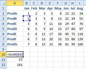
The simplest reference is when you point to a single cell.
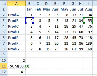
If you sum two cells and separate those cells with a comma, then Excel will add up the two individual cells. Below, the formula is adding B3 and I3.
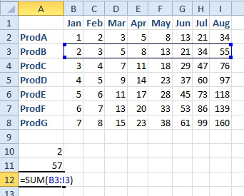
When you list two cells and separate those cells with a colon, Excel will add up everything between and including the two cells.
Everyone using Excel has undoubtedly seen the references as shown above.
There is a different type of reference called an intersection. In this case, you would separate two ranges by a space instead of a comma. =SUM(C2:C8 B3:I3) would give you all of the cells in common between the two ranges.
To see a useful example, it would help to add many range names to the worksheet. Follow these steps:
1. Select A1:I8.
2. From the Formulas tab, select Create From Selection.
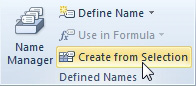
3. Leave Top Row and Left Column checked. Click OK.
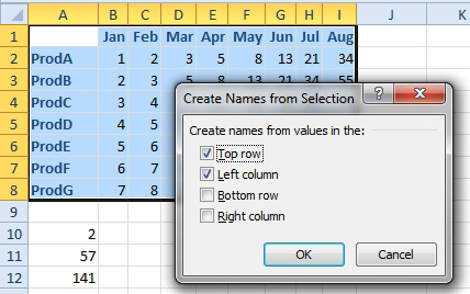
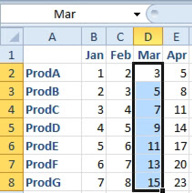
This will create 15 new range names. The name of Mar now refers to D2:D8. The name of ProdG now refers to B8:I8. This itself is a cool trick.
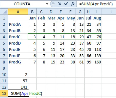
Going back to the intersection operator, a formula of =SUM(Apr ProdC) will return the intersection of the two ranges. This provides an interesting way to do a two-way loookup.
You can use Data Validation to add a dropdown to two cells. In one cell, someone could select a product. In another cell, someone could select a month.
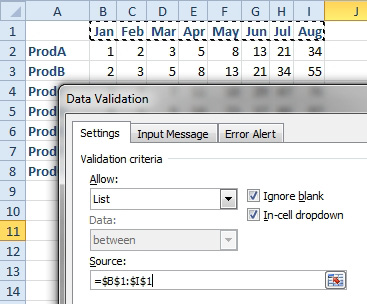
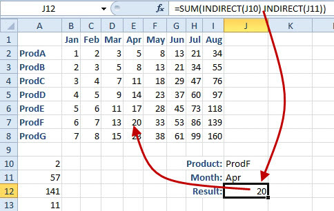
The INDIRECT(J10) function tells Excel to go to J10 and the name of a range will be found in that cell. In the figure below, the formula in J12 is getting the intersection of ProdF and Apr, which returns the value of 20.
This article is an excerpt from Power Excel With MrExcel
Title photo by Ryan Besgrove on Unsplash