What Happened to Multiple Consolidation Ranges in Pivot Tables?

February 09, 2023 - by Bill Jelen

Problem: I read your book Pivot Table Data Crunching, which describes an awesome trick for spinning poorly formatted data into transactional data for pivot tables. The trick requires you to choose Multiple Consolidation Ranges from Step 1 of the PivotTable and PivotChart Wizard. However, Microsoft seems to have eliminated the wizard in Excel 2007, so now how can I select Multiple Consolidation Ranges?

Strategy: Although the PivotTable and PivotChart Wizard has been removed from the ribbon, you can still get to the old wizard:

1. Type Alt+D followed by P.
2. The PivotTable and PivotChart Wizard will appear, complete with new artwork.

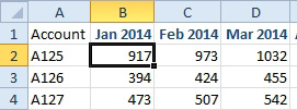
Additional Details: Using multiple consolidation ranges can help when your data is not properly formatted for pivot tables. Below, the data has been summarized with months going across the columns. Each year is on a different worksheet. All of the worksheets have products along column A, but the list of products differs from year to year.

This data has account down the left column and months across the top. — Figure 1006. Months going across rarely works for pivot tables.

1. Type Alt+D+P to open the old PivotTable Wizard.
2. In Step 1 of the wizard, choose Multiple Consolidation Ranges. Click Next.
3. In Step 2a, choose I Will Create the Page Fields. (You don’t have to create page fields, you just don’t want Excel to create page fields.)
4. Click Next.
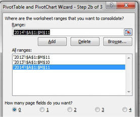
5. In Step 2b, choose the range on the first sheet. Click Add.
6. Repeat Step 5 for each additional worksheet. The dialog should look like below.
7. Click Finish.

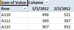
In the old days, you could choose Multiple Consolidation Ranges for a pivot table. This figure shows the old Pivot Table Wizard Step 2B of 3, where you would specify all the ranges to consolidate. — Figure 1007. Consolidate data from three worksheets.

Excel will create a pivot table that summarizes all the worksheets. The fields have the strange names Row, Column, and Value.

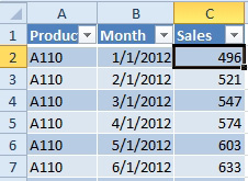
The resulting pivot table has dates across the top, accounts down the side, but the field names are Row and Column. — Figure 1008. The worksheets are combined into one pivot table.

As you read in “See Detail Behind One Number in a Pivot Table,” you can double-click any cell in a pivot table to drill down to see all the records in that cell. Here is the amazing trick: If you double-click the Grand Total cell in the pivot table, Excel will produce a new worksheet with all your data in detail format, as shown below. All you have to do is rename the headings from Row, Column, and Value to Product, Month, and Sales.

After drilling down on the Grand Total cell, you get Product in A, Date in B, Sales in C. — Figure 1009. Double-click the Grand Total to get a data set combining data from all worksheets.

This article is an excerpt from Power Excel With MrExcel

Title photo by Susan Q Yin on Unsplash