Using Variable Ranges for Unique Counts

January 29, 2018 - by Bob Umlas

Say that you want to be able to count unique items from a list, but with a twist. And say you’re working with this worksheet:

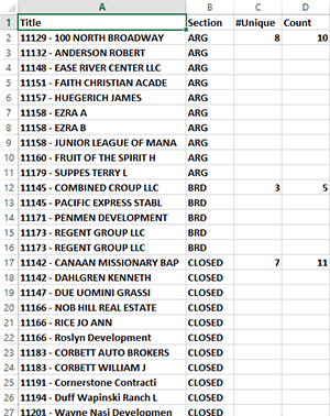
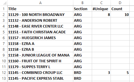
Column D counts the number of rows in each of the sections from column B, and column C counts the number of unique sections based on the first five characters of column A for that section. Cells B2:B11 contain ARG, and you can count eight unique items in the first five characters of A2:A11 because A7:A9 each contain 11158, so the two duplicates are not counted. Similarly, the 5 in D12 tells you there are five rows for BRD, but within rows 12:16, there are three unique items of the first five characters, since 11145 is repeated and 11173 is repeated.

But how do you tell Excel to do this? And what formula could you use in C2 that could be copied to C12 and C17?

The simple counting formula in D2, =COUNTIF(B:B,B2), counts the number of times B2 (ARG) exists in column B.

You use a helper column to isolate the first five characters of column A, as in this figure:

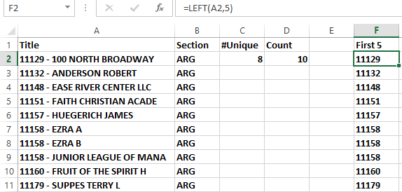
Next, you need to somehow indicate that for ARG, you’re only interested in cells F2:F11 to find the number of unique items. In general, you would find this value by using the array formula shown in this figure:

You use cell C3 temporarily just to show the formula; you can see that it’s not present in C3 in previous figures. (You’ll learn shortly how this formula works.)

So what’s the formula in C2, C12, and C17? The surprising (and cool) answer is shown in this figure:

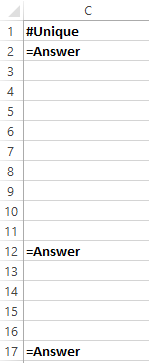
Whoa! How does this work?

Take a look at Answer in the defined names in this figure:

It’s the same formula from an earlier figure, but instead of using the range F2:F11, it uses a range named Rg. Also, the formula was an array formula, but named formulas are treated as if they are array formulas! That is, =Answer is not entered with Ctrl + Shift + Enter but is simply entered as usual.

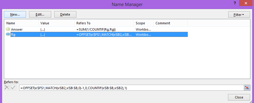
So how is Rg defined? If cell C1 is selected (which is an important step for understanding this trick), then it’s defined as in this figure:

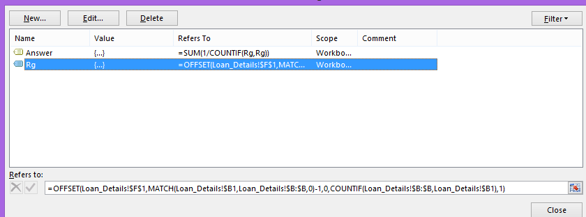
That’s =OFFSET(Loan_Details!$F$1,MATCH(Loan_Details!$B1,Loan_Details!$B:$B,0)-1,0,COUNTIF(Loan_Details!$B:$B,Loan_Details!$B1),1).

Loan_Details is the name of the sheet, but you can look at this formula without the long sheet name. An easy way to do this is to temporarily name the sheet something simple, like x, and then look again at the defined name:

This formula is easier to read!

You can see that this formula matches $B1 (note the relative reference to the current row) against all of column B and subtracts 1. You subtract 1 because you’re using OFFSET from F1. Now that you know about the formula for C, take a look at the one for C2:

The MATCH($B2,$B:$B,0) part of the formula is 2, so the formula (without the reference to the sheet name) is:

=OFFSET($F$1,2-1,0,COUNTIF($B:$B,$B2),1)

or:

=OFFSET($F$1,1,0,COUNTIF($B:$B,$B2),1)

or:

=OFFSET($F$1,1,0,10,1)

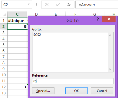
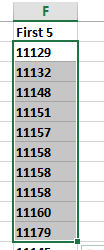
Because COUNTIF($B:$B,$B2) is 10, there are 10 ARGs. This is range F2:F11. As a matter of fact, if cell C2 is selected and you press F5 to go to Rg, you see this:

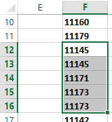
If the starting cell were C12, pressing F5 to go to Rg produces this:

So now, with Answer defined as =SUM(1/COUNTIF(rg,rg)), you’re all done!

Let’s look more closely at how this formula works, using a much simpler example. Normally, the syntax for COUNTIF is =COUNTIF(range,criteria), such as =COUNTIF(C1:C10, "b") in this figure:

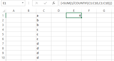
This would give 2 as the number of b’s in the range. But passing the range itself as the criteria uses each item in the range as the criteria. If you highlight this portion of the formula:

and press F9, you see:

Each item in the range is evaluated, and this series of numbers means there’s one a and there are two b’s, three c’s, and four d’s. These numbers are divided into 1, giving 1, ½, ½, ⅓, ⅓, ⅓, ¼, ¼, ¼, ¼, as you can see here:

So you have 2 halves, 3 thirds, 4 fourths, and 1 whole, and adding them up yields 4. If an item were repeated 7 times, then you’d have 7 sevenths and so on. Pretty cool! (Hats off to David Hager for discovering/inventing this formula.)

But hold on a minute. As it stands, you have to only enter this formula in C2, C12, and C17. Wouldn’t it be better if you could enter it in C2 and fill down and only show it in the correct cells? In fact, you can do this. You can modify the formula in C2 to be =IF(B1<>B2,Answer,""), and when you fill that down, it does the job:

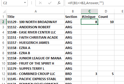
But why stop here? Why not make the formula into a named formula, as shown here:

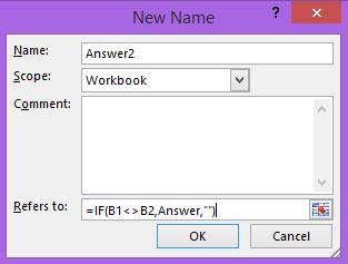
For this to work, cell C2 must be the active cell (or the formula would need to be different). Now you can replace column C’s formulas with =Answer2:

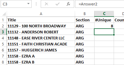
You can see that C3 has =Answer2, as do all the cells in column C. Why not continue this in column D? The formula in D2, after also applying the comparison to B1 and B2, is shown here:

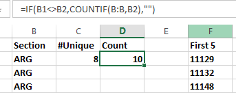
So if you keep cell D2 selected and define another formula, say Answer3:

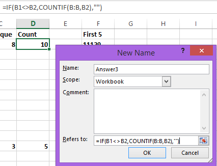
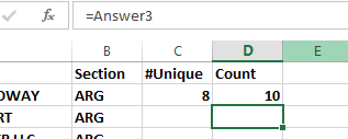
then you can enter =Answer3 in cell D2 and fill down:

Here’s the top part of the worksheet, with formulas showing, followed by the same screenshot with values showing:

When other people try to figure this out, they might scratch their head at first!

Title Photo: PublicDomainPictures / pixabay

This guest article is from Excel MVP Bob Umlas. It is from the book, More Excel Outside the Box. To see the other topics in the book, click here.