Use Real Dates

June 13, 2022 - by Bill Jelen

Problem: I hate Excel dates. I try to do a calculation and I get a number like 43148. Or I try to calculate the number of days between an invoice and a payment and I get an answer like January 15, 1900.

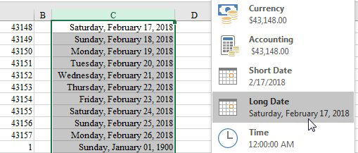
Strategy: It will take five minutes to understand how Excel stores dates. Open a blank worksheet. Type a number in the range of 42000 to 44000 in cell A1. Select that cell. Hold down the Ctrl key while you drag the fill handle down for several cells. At the bottom of the list, enter a 1. Over in column C, enter =A1 and copy it down. You should have two identical columns of numbers.

Select column C. On the Home tab, open the General dropdown and choose Long Date. Column C will change to show dates in the modern era, plus January 1, 1900.

A column of numbers around 43000 formatted as dates will show dates in the 2018 era. — Figure 512. Format the numbers as dates.

You haven’t changed the value stored in column C. Cell C1 still contains 43148. You have told Excel to treat the cell as a date and so it calculates a weekday, month, day, and year when applying the formatting.

Additional Details: Excel stores dates as the number of days elapsed since January 1, 1900. Assuming that you are reading this book in the 2017–2021 timeframe, whenever you see a number in the 42700–44600 range, you might be seeing a date cell that is not formatted as a date.

When I say that you should use “real” dates, I mean to store a number like 43148 in the cell and use numeric formatting to display that number as a date. The main advantages of real dates are that you can easily change the format of the date, and you can easily do any calculations that you need with the dates. You can not do calculations when you have dates that are stored as text.

Gotcha: While Excel is really fast at converting 43148 to a month, day, year, it does a notoriously bad job of deciding whether to format the result of a formula as a number or as a date. Here are two examples:

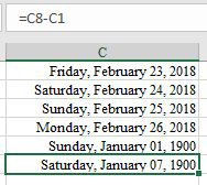
Go to the bottom of your dates in column C and calculate =C8-C1. This formula should calculate the number of elapsed days between the two dates. The correct answer is 7. Excel gets the correct answer, but because that column was previously formatted to show long dates, you will see the 7 converted to Saturday, January 7, 1900.

=C8-C1 is supposed to show 7 days have elapsed. But Excel formats the answer as date and it shows as January 7, 1900. — Figure 513. The correct result of 7 is incorrectly formatted as a date.

To solve the problem, go back to the numeric formatting dropdown on the Home tab and choose Number. The result will now appear as 7 or 7.00. The problem in this case was that you entered a formula that should return a number in a column that had previously been formatted to show dates.

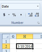
A similar problem is that sometimes, you might enter a function that should return a date. The formula bar will show the formula, and the worksheet cell will show the serial number.

A WORKDAY function always returns a date, but Excel tends to format it as a number instead of a date. Here, =WORKDAY(A1,15) return 41708. — Figure 514. Excel didn’t think to format this as a date.

To solve the issue, format the cell as a short date.

Here, the problem was that you entered a formula that should return a date in a cell that was formatted as General.

Gotcha: 80% of the time, Microsoft takes control and automatically formats your cell with the correct format.

Format the WORKDAY cell as a date and you have 3/10/2014. — Figure 515. Change from General format to Short Date.

Go to a blank cell and enter =DATE(2018,7,1) and Excel will automatically format that cell to convert the serial number to a short date. But, this trick does not work with any function that originated in the old Analysis ToolPak.

Bottom line: Be prepared to have to change the formatting, either from General to a Date or from a Date back to Number.

This article is an excerpt from Power Excel With MrExcel

Title photo by Towfiqu barbhuiya on Unsplash