Use Formulas for Chart Labels in Excel
July 18, 2023 - by Bill Jelen

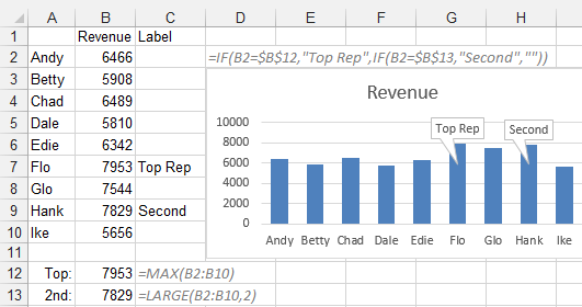
Excel 2013 introduces a new feature where the chart labels can come from other cells on the worksheet. In the Figure below, formulas in column C build a label to identify the largest and second largest sales amount.

Here are the steps to assign the labels from cells:
1. Select the data and Insert, Recommended Chart, OK.
2. Use the Plus icon to the right of the chart. Add a checkmark to Data Labels.
-
3. Plus Icon, hover to right of Data Labels. Click Triangle, choose Data Callout.
4. Plus, Data Labels, Triangle, More Options.
5. Click the 3-Column chart icon in the Format Data Labels Task Pane.
6. Click on Label Options.
7. Checkmark Value From Cells.
8. Excel will ask you to highlight the range. In this case, it is C2:C10.
9. Uncheck Category Name and Value.
This article is an excerpt from Power Excel With MrExcel
Title photo by Helena Hertz on Unsplash
