Use Consolidation to Combine Two Lists

October 21, 2022 - by Bill Jelen

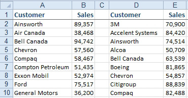
Problem: Jerry and Tina each compiled sales figures from paper invoices. I need to combine Jerry and Tina’s list into a single list. Some customers are in both lists.

Introducing the Consolidate feature. In this example, you have two lists with Customer in the first column and Sales in the second. Some customers are in both lists, most are only in one list. You want to combine the lists. If the same customer appears in both lists, total their values. — Figure 764. Combine the lists into a single list.

Strategy: Excel offers a great tool for consolidating data. Here’s how you use it:

1. Move the cell pointer to a blank area of the worksheet. You will need a blank area with several rows and a few columns.
2. Select Data, Consolidate.
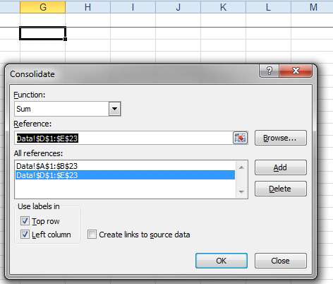
3. Make sure that both boxes under Use Labels In are checked. This means that Excel relies on the headings to be the same and that the customer field is in the left column of each range.
4. Put the cell pointer in the Reference field. Click the Collapse button at the right end of the Reference field. With the mouse, select the first range: A1:B23. Click the Collapse button again to return to the Consolidate dialog.

Note: There are times when you will want to consolidate just a single range of data. This would be effective if you needed to combine duplicate customers from one list. However, in this example, you need to combine two lists.

5. Click the Add button to move the first reference from the Reference field to the All References box.
6. After the first reference is added to the All References box, click the Collapse button again to specify the second reference.
7. Use the mouse to select D1:E23. Click the Collapse button to return to the Consolidate dialog. Click the Add button to add the reference to the All References list. The Consolidate dialog should appear as below

In the Consolidate dialog, the Function is chosen to be Sum. Specify the address for each list and click the Add button to get the complete list of references in the All References box. Near the bottom left, choose Top Row and choose Left Column. Do not select Create Links to Source Data. Click OK. — Figure 765. Make sure both ranges are in the All References box.

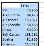
8. Choose OK. In a few seconds, Excel will return a brand new list that extends down and to the right from your starting cell. The list will contain one instance of each customer along with the total revenue from the customer.

The results of Consolidate always have a blank top left cell. The word Sales is to the right of the blank cell. In each row that follows, you have a customer and the total revenue for that customer. — Figure 766. Excel combines the two lists into a single list.

Gotcha: The new list is not in any sequence. You can see that it kind of starts out in the sequence of the first list but then randomly inserts customers from the second list. You will probably want to sort the list alphabetically or by revenue. However, Excel always fails to fill in the label in the upper-left corner of the consolidation. If you want to sort the result, you need to type the word Customer in cell G2.

Additional Details: The Function box in the Consolidate dialog offers many functions other than SUM. For instance, if you want to find the largest purchase by each customer, you can use the MAX function.

Gotcha: The results of the consolidation are all static values. If you change an item in the original list, the consolidation will not automatically update. This is good because it allows you to delete the original two lists and keep just the new list.

This article is an excerpt from Power Excel With MrExcel

Title photo by Алекс Арцибашев on Unsplash