
Use a Pivot Table When There Is No Numeric Data
February 06, 2023 - by Bill Jelen

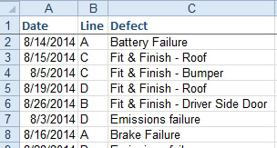
Problem: My data set contains a list of manufacturing defects found in quality inspection for one month. I have fields for date, manufacturing line, and defects. There are no numeric fields. Can I analyze this data with a pivot table?
Strategy: You can use the COUNT function to perform a Pareto analysis. Here’s how:
1. Create a pivot table. Choose the Defect field, and Excel will automatically add it to the Row Labels drop zone.
2. Drag the Defect field from the top of the Field List dialog to the Values drop zone. Excel will add the Defect field to the pivot table twice. Because Defect is a text field, Excel automatically decides to count the number of occurrences.
-
3. Sort the pivot table by Count of Defect, descending. You now have a list of each defect and how often it occurred.
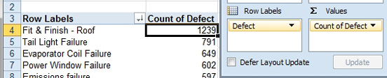
4. Study the pivot table to find defects with the most problems. The fit of the roof and tail lights are causing the most problems.
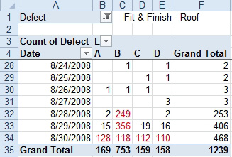
5. Change the pivot table to have Dates in the Row Labels and Line in the Columns. Move Defect from the Row Labels to the Report Filter.
6. Choose Fit & Finish – Roof from the Report Filter dropdown in B1. This was the defect that occurred most often.
Results: As shown below, the defect was happening a few times each day until the 28th of the month. On the 28th, line B began having problems. On the 29th, the problem began appearing in lines A, C, and D. By the 30th, all four lines were having massive problems. This doesn’t look like a problem with an isolated employee, so you should probably see if a new batch of material started being used on the 28th.
This article is an excerpt from Power Excel With MrExcel
Title photo by Surendran MP on Unsplash