
Use a Pivot Table to Compare Two Lists
February 03, 2023 - by Bill Jelen

Problem: I have two lists of data. One is from a forecasting system. One is from our order entry system. I want to compare both list. Although both lists happen to have twenty customers, they are not the same twenty customers.

The pivot table method is far easier than using two columns of MATCH or VLOOKUP.
Strategy: You need to copy the two lists into a single list, with a third column to indicate whether the forecast is from this week or last week. Then you create a pivot table, and the new, deleted, and changed forecasts will be readily apparent. Follow these steps:
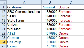
1. Add the heading Source in C1. Select C2:C21, type Forecast and press Ctrl+Enter to fill column C with the word Forecast.
-
2. Change the heading in B1 to be Amount.
3. Cut D2:E21 and paste just below the first list. Type Orders next to all of the List 2 records.
4. Create a pivot table. Put Customer in the Row Labels, Source in Column Labels, and Amount in the Values area.
5. Right-click the Grand Total heading and choose Remove Grand Total.
As shown here, you will have a comparison of the two lists.
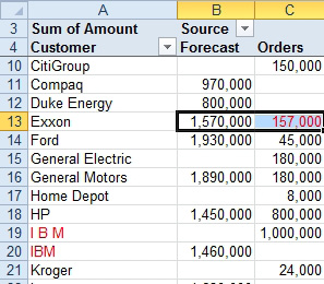
In this view, you can spot many interesting facts. It looks like the IBM misspelling in row 20 is causing problems. That forecast is most likely associated with the order in row 19. I would also be concerned with the Exxon forecast and order in row 13. Did the sales rep accidentally type an extra zero when submitting his forecast?
This article is an excerpt from Power Excel With MrExcel
Title photo by Vanesa Giaconi on Unsplash