Troubleshooting VLOOKUP
July 25, 2017 - by Bill Jelen

Excel VLOOKUP is powerful, but it won't work when you have specific situations. Today, a look at how to troubleshoot VLOOKUP.
VLOOKUP is my favorite function in Excel. If you can do VLOOKUP, you are able to solve many problems in Excel. But there are things that can trip up a VLOOKUP. This topic talks about a few of them.
But first, the basics of VLOOKUP in plain English.
The data in A:C came from the IT department. You asked for sales by item and date. They gave you Item number. You need Item Description. Rather than wait for the IT department to re-run the data, you find the table shown in column F:G.

You want VLOOKUP to find the item in A2 while it searches through the first column of the table in $F$3:$G$30. When VLOOKUP finds the match in F7, you want VLOOKUP to return the description found in the second column of the table. Every VLOOKUP that is looking for an exact match has to end in False (or zero, which is equivalent to False). The formula below is set up properly.
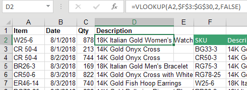
Notice that you use F4 to add four dollar signs to the address for the lookup table. As you copy the formula down column D, you need the address for the lookup table to remain constant. There are two common alternatives: You could specify the entire columns F:G as the lookup table. Or, you could name F3:G30 with a name such as ItemTable. If you use =VLOOKUP(A2,ItemTable,2,False), the named range acts like an absolute reference.
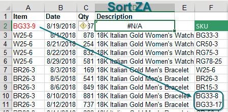
Any time that you do a bunch of VLOOKUPs, you need to sort the column of VLOOKUPs. Sort ZA, and any #N/A errors will come to the top. In this case, there is one. Item BG33-9 is missing from the lookup table. Maybe it is a typo. Maybe it is a brand-new item. If it is new, insert a new row anywhere in the middle of your lookup table and add the new item.
It is fairly normal to have a few #N/A errors. But in the figure below, exactly the same formula is returning nothing but #N/A. When this happens, I see if I can solve the first VLOOKUP. You are looking up the BG33-8 found in A2. Start cruising down through the first column of the lookup table. As you can see, the matching value clearly is in F10. Why can you see this, but Excel cannot see it?
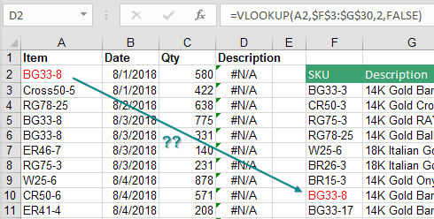
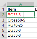
Go to each cell and press the F2 key. Here is F10. Note that the insertion cursor appears right after the 8.

Here is cell A2 in Edit mode. The insertion cursor is a couple of spaces away from the 8. This is a sign that at some point, this data was stored in an old COBOL data set. Back in COBOL, if the Item field was defined as 10 characters and you only typed 6 characters, COBOL would pad it with 4 extra spaces.
The solution? Instead of looking up A2, look up the TRIM(A2).

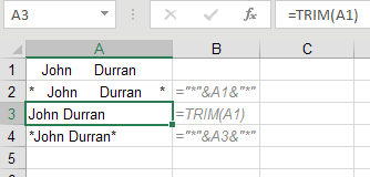
The TRIM() function removes leading and trailing spaces. If you have multiple spaces between words, TRIM will convert them to a single space. In the figure below there are spaces before and after both names in A1. =TRIM(A1) removes all but one space in A3.
By the way, what if the problem had been trailing spaces in column F instead of column A? Add a column of TRIM() functions to E, pointing to column F. Copy those and paste as values in F to make the lookups start working again.
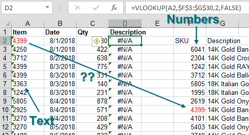
The other very common reason that VLOOKUP won’t work is shown here. Column F has real numbers. Column A has text that looks like numbers.
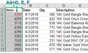
Select all of column A. Press Alt + D, E, F. This does a default Text to Columns and will convert all text numbers to real numbers. The lookup starts working again.
Watch Video
- VLOOKUP solves many problems
- Common VLOOKUP problems:
- If VLOOKUP starts out working, but #N/A becomes more prominent: forgot $ in lookup table
- A few #N/A: items missing from the table
- None of the VLOOKUP work: check for trailing spaces
- Remove trailing spaces with TRIM
- Numbers and numbers stored as text
- Select both columns and use Alt + D E F
- Episode includes a joke that both accountants and IT people find funny, but for different reasons
Video Transcript
Learn Excel from MrExcel podcast, episode 2027 - Troubleshooting VLOOKUP!
Alright, podcasting this entire book, click the “i” on the top-right hand corner to get to the playlist!
VLOOKUP Is my favorite function in all of Excel, and I always tell this joke in one my seminars, and it gets a laugh whether you're an IT person or not an IT person. I always say “Well look, we have this data set here on the left, and I can look at that data and tell that data came from the IT department because it's exactly what I asked for, but not really what I needed. I asked for item date and quantity, and they gave me item number date and quantity, but they didn't bother to give me description, right?” And the accountants always laugh at this, because this happens to them all the time, and the IT guys are like “Well, I gave you what you asked for, it's not my fault!” So they both think it's funny for different reasons so, you know, and the IT guy is busy, he can't get back to rewriting the query, so we have to do something to rescue this ourselves.
And so this little table I copied from somewhere else in my computer, in plain English, what VLOOKUP does is says “Hey, we have an item number W25-6.” We have a table here, I want to cruise down through the first column of the table until I find that item number, and then return something from that row. Alright, in this case, what I want is the 2nd column from that row. And then at the end of every VLOOKUP we have to put either FALSE or 0. Now right here, after I choose the range, I'm going to press the F4 key, and then I want the 2nd column and then FALSE for an exact match. Don't ever choose approximate match, never, never! It's not an approximate match, it's a very special thing, it doesn't work all the time. If you like to restate your numbers to the Securities and Exchange Commission, by all means feel free to use ,TRUE or just leave the ,FALSE off. But every VLOOKUP that you ever create should end in ,FALSE or ,0, 0 is shorter than FALSE, you're supposed to put a FALSE there, but a 0 is the same thing as FALSE.
Alright now, troubleshooting, first thing, when you do a whole bunch of VLOOKUPs, it's very normal to have a couple of #N/As, right? And I Always find the #N/A’s by going Data, Z-A, that brings the #N/As to the top, right there, BG33-9, either that's a typo or it's a brand-new item, alright, and we got to figure it out. So over here to the right I have the new data, I will cut that, and then Alt+I E D, insert those cells in the middle, it does not have to be alphabetic, this table does not have to be sorted. When you're using the ,FALSE version, the table isn't- you can just put it anywhere you want, I didn't put at the end because I didn't have to rewrite the formula, I just want the formula to work. Alright, so a couple of #N/A’s, extremely, extremely normal, but check this out.
When you start out with answers that work, but then the #N/A’s start to appear slightly frequently, and then eventually they appear all the way down, that's a sure sign that you didn't lock down the table reference. Alright see, so here the table is moving as I copy the formula down, right, and so I'm getting lucky in hitting a few that were at the end of the list. But eventually I get down to the point where it's looking over here in completely blank cells, and of course nothing is being found. Alright, so that's the first thing, you get a couple that work, a few #N/A’s, a couple more that work, and then all #N/A’s the rest of the way - sure sign that you didn't put the $ in.
Just go back, F2 for Edit mode, select the colon, press F4, that puts all the $ in, double-click to shoot that down, and things start to work again, alright. Next one, exact same formula, the formula is perfect, BG33-8 see, we're getting none of that right. Alright, so I go look, BG33-8, hey, there it is, it's right there, it's in red, I should have seen it! So I come to this one on the right-hand side, I press F2, and I watch the flashing insertion point, and see, it's right after the 8, like that, and then I come over here and I press F2, there are some trailing spaces there. This is very, very common back in the days of COBOL, they would say “You know, look, we're going to give you 10 spaces for item number, and if you don't type all 10 spaces they will fill the spaces.” And so this is very common, and the great solution here is to get rid of those leading and trailing spaces with the TRIM function. Instead of A2 use the TRIM(A2), double-click to shoot that down, alright, still the BG33-9 is back in the other table.
Alright, just so you understand how TRIM works, so I typed a bunch of spaces, John, a bunch of spaces, Durran, and a bunch of spaces, and then I concatenated a * before and after so you can see what it looks like. When I ask for the TRIM(P4), we get rid of all the leading spaces, all the trailing spaces, and then the multiple interior spaces are reduced down to one space. Alright, so you can see, kind of visualize there, that they're getting rid of leading and trailing spaces, any doubled-up spaces of the middle become a single space like that. So TRIM, great, great tool in your arsenal, alright, here's another really common one.
If it's not the trailing spaces, then the most common thing that I've seen, is where over here we have true numbers, and here we have numbers stored as text. And VLOOKUP won't see that as a match, even though 4399, this is a number, this is text, doesn't work. Fastest way to convert a column of text to numbers, select the column, 3 letters in sequence, Alt D E F, and all of a sudden, our VLOOKUPs start to work again, great, great tip from about 1500 podcasts ago. Alright, so those are the most common VLOOKUP problems, either you forgot the $, or you have trailing spaces, or you have numbers and numbers stored as text. All of these tips are in this book “MrExcel XL”, click ihe “i” on the top-right hand corner, you can buy the book.
Alright, quick recap: VLOOKUP solves many problems, if a VLOOKUP starts working but #N/A! becomes more prominent, you forgot to put the $ in the lookup table. If there's a few #N/A’s, it's just items missing from the table. If none of the VLOOKUPs work and it’s text, check for trailing spaces, you can use the TRIM function. If you have numbers and numbers stored as text, select either column, the one that has the text, then do Alt D E F have to all those back to numbers.
Alright well hey, I want to thank you for stopping by, we'll see you next time for another netcast from MrExcel!
Download File
Download the sample file here: Podcast2027.xlsx
Title Photo: radekkulupa / Pixabay
