Total Numbers From Data Alt-Entered

February 23, 2023 - by Bill Jelen

Problem: I work for a bunch of people who don't know how to use Excel. They insist on treating an Excel like it is Microsoft Word, using Alt+Enter to put multiple things in one cell.

Cell A2 is for cost center 1001. In cell B2, four lines items appear, each with a label a dash, and a number:
Rent - 1000
Telephone - 500
Utilities - 225
Security - 125
Row 3 has similar data for cost center 1002. — Figure 1018. Cell B2 is essentially a Word document.

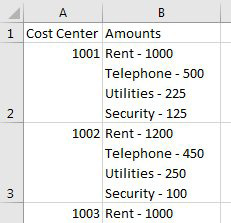
Strategy: Power Query can handle this. The Split Column feature, which started out similar to Text to Columns in Excel has a new twist: it can split a cell and move each value to a new row instead of a new column.

Follow these steps:

1. Format the original data as a table using Ctrl+T
2. On the Data Tab, choose From Table/Range. Wait for the Power Query Editor to load.
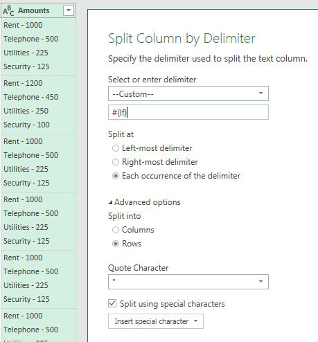
3. Select the Amounts column in Power Query. On the Home tab, choose Split Column, By Delimiter.
4. For the delimiter, choose Custom. Leave the delimiter box empty for now.
5. Open the Advanced Options.
6. Choose to Split Into Rows
7. Choose the box for Split Using Special Characters.
8. Click into the Delimiter box. Use the Insert Special Character drop-down and choose Linefeed. Power Query inserts a code for linefeed inthe delimiter box.
9. Click OK.

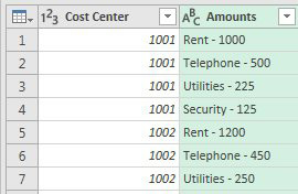
In Power Query, use Split Column by Delimiter. Choose Custom as the Delimiter. Using the button at the bottom for Insert Special Character, select Linefeed. This appears in the delimiter bow as #(lf). In Advanced Options, choose Split Into Rows. — Figure 1019. The Split Columns feature runs circles around Text to Columns.

At this point, the data is half clean..

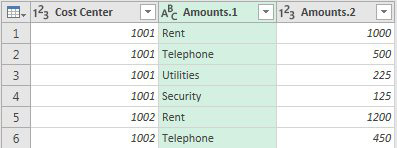
After splitting to Rows, you have four rows for Cost Center 1000 in column A, then column B still says Rent - 1000, Telephone - 500, but these are now in separate rows. — Figure 1020. Each item is in it's own row.

Choose the Amounts column and Split Column by Delimiter of " - ". You now have three columns.

After splitting Column B by the dash, you get Amounts.1 with the name of the Expense Item and Amounts.2 with the actual amount. — Figure 1021. You could create a pivot table from this.

While you are likely happy at this point and ready to head back to Excel, you can further summarize the data in Power Query.

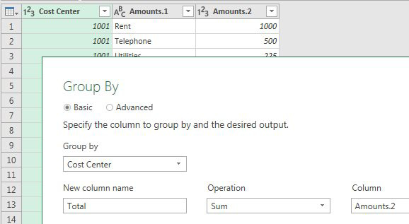
Choose the Cost Center column. On the Transform tab, choose Group By. Fill out the Group By dialog as shown:

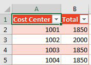
Choose the Cost Center column and then Transform, Group By. In the Group By dialog, choose Basic, Group by Cost Center, New Column Name is Total, Operation is Sum, Column is Amounts.2. — Figure 1022. Reduce the data to one line per cost center.

After you close and load, you will end up with a new worksheet with a summary by cost center.

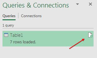
The result is a new table with Cost Center in A, Total in B. The four lines for Cost Center 1001 now appear as one row, with a total of 1850. — Figure 1023. Use VLOOKUP in the original table to grab the totals from this.

Any time that you type new numbers in the original data, use the Refresh icon to update the summary table.

In the Queries & Connections pane, Table1 says 7 rows loaded. Make the pane wider, and click the Refresh icon that appears at the right edge of the pane. — Figure 1024. The Refresh icon is hidden unless you make the panel wider.

This article is an excerpt from Power Excel With MrExcel

Title photo by Volodymyr Hryshchenko on Unsplash