
Three Methods of Entering Formulas
November 18, 2021 - by Bill Jelen

Problem: I’d like to enter formulas faster. What are the three ways of entering simple formulas?
Strategy: There are three ways of entering formulas. Learning the arrow key method will dramatically improve your efficiency with Excel. This topic will compare all three methods.
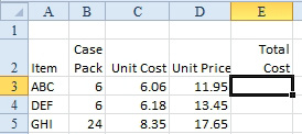
Say that you want to calculate total cost in E3 as the case quantity in B3 multiplied by the unit cost in C3.
One way to make this calculation is to simply type the formula:
-
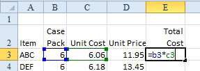
1. Put the cell pointer in E3 and type =b3*c3 and then press Enter.
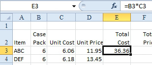
2. The formula will calculate. You will see the original formula in the formula bar above E1. The worksheet will show the result of the calculation.
This method is great for short functions that require only a few keystrokes. However, this method gets complicated when you are dealing with complex formulas.
Alternate Strategy: Another way to enter calculations is to use the arrow keys. Anyone who was using spreadsheets in the days of Lotus 1-2-3 often used this method. When you have mastered this method, it is very fast and very intuitive. Here’s how it works:
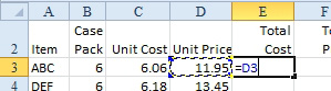
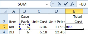
1. Move the cell pointer to E3 and type an equals sign to let Excel know that you are about to enter a formula.
2. Press the Left Arrow key. As shown here, a dotted border surrounds the cell to the left of E3. Excel starts to build the formula
=D3.
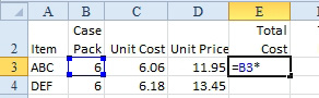
3. Press the Left Arrow key two more times. Your provisional formula is now
=B3.
4. Press * on either the keyboard or the numeric keypad. The dotted border will disappear from B3 and be replaced by a solid-colored border. Pressing any operator key, such as +, -, *, or /, tells Excel that you are moving on to the next part of the formula. At this point, focus returns to cell E3.
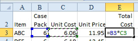
5. Press the Left Arrow key two times. The dotted border reappears. You now have a provisional formula of
=B3*C3.
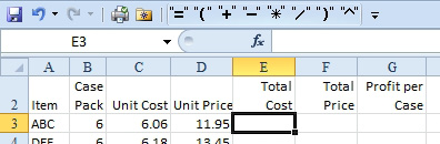
6. Press Enter. The formula will calculate. You will see the original formula in the formula bar above E1. The worksheet will show the result of the calculation.
Additional Details: With this method, you never have to type cell references. You merely point to them using the arrow keys. If you are building formulas that are based on cells near the formula cell, you can enter them very quickly using this method.
Although I used several paragraphs and five screen shots to show this method, it required only eight keystrokes, many of which were repeats of the same keystroke. Further, because you are allowed to start a formula with a plus sign instead of an equals sign, you can enter the entire formula using the keys on and around the numeric keypad on a desktop computer (that is, +←←←*←←Enter).
Alternate Strategy: Another way to enter calculations in Excel is to use the mouse. Normally, people use the keyboard to type the equals sign, math operators, and enter and the mouse to click on cell references. Moving your hand from the mouse to the keyboard takes a lot of time and dramatically slows the entry of formulas. Adding a few icons to your Quick Access toolbar can dramatically speed formula entry. Follow these steps.
1. Using steps from "Make Your Most-Used Icons Always Visible", add icons for equals, plus, minus, multiply, divide, exponents, left parenthesis, and right parenthesis to the Quick Access Toolbar. These icons are found in the “Commands Not in the Ribbon” category.
2. Right-click the Quick Access Toolbar and choose Show Quick Access Toolbar Below the Ribbon.
3. Start in cell E3. Click the equals sign icon.
4. Click on cell B3 with the mouse.
5. Click on the * sign in the QAT
6. Click on cell C3 with the mouse.
7. Click the checkmark icon to the left of the formula bar to accept your formula.
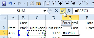
8. The formula will calculate. You will see the original formula in the formula bar above E1. The worksheet will show the result of the calculation.
There are three basic methods for entering formulas in Excel. Using the easiest method for the situation can radically improve your efficiency.
This article is an excerpt from Power Excel With MrExcel
Title photo by Charlota Blunarova on Unsplash