The VLOOKUP Slayer: XLOOKUP Debuts Excel
August 28, 2019 - by Bill Jelen

The whole purpose of XLOOKUP is to find one result, find it quickly, and return the answer to the spreadsheet.
At Noon today, Microsoft began slowly releasing the XLOOKUP function to some Office 365 Insiders. The main benefits of XLOOKUP:
- Can find the last match!
- Can look to the left!
- Defaults to an exact match (unlike VLOOKUP which defaults to True for the 4th argument)
- Defaults to not support wildcards, but you can explicitly allow wildcards if you want them
- Has all the speed improvements released to VLOOKUP in 2018
- No longer relies on Column Number, so it won't break if someone inserts a column in the middle of the lookup table
- Performance improvement because you are only specifying two columns instead of the whole lookup table
- XLOOKUP returns a range instead of VLOOKUP returning a value
Introducing XLOOKUP
The XLOOKUP Syntax is:
XLOOKUP(Lookup_Value, Lookup_Array, Results_Array, [Match_Mode], [Search_Mode])
The choices for Match_Mode are:
- 0 Exact Match (default)
- -1 Exact Match or Next Smaller
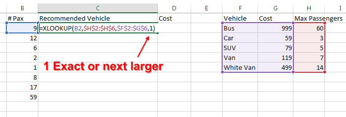
- 1 Exact Match or Next Larger
- 2 Wildcard Match
The choices for Search_Mode are
- 1 first to last (default)
- -1 last to first
- 2 binary search, first to last (requires lookup_array to be sorted)
- -2 binary search, last to first (requires lookup_array to be sorted)
Replacing a Simple VLOOKUP
You have a lookup table in F3:H30. The lookup table is not sorted.
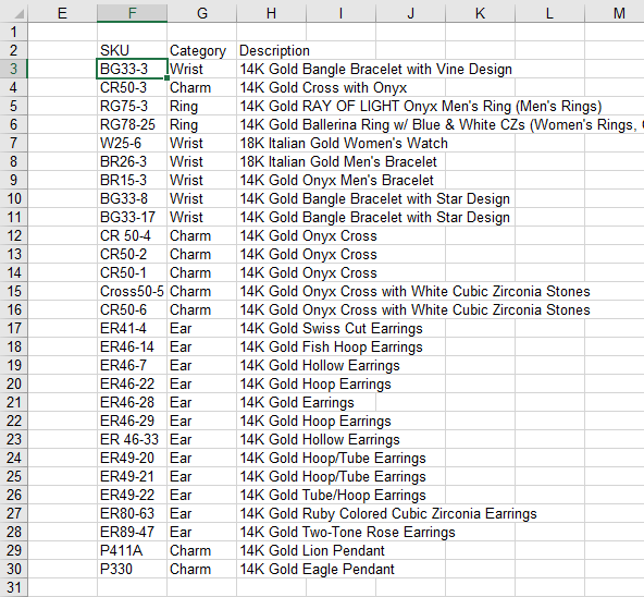
You want to find the description from the table.
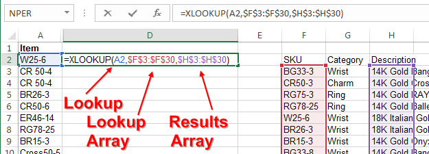
With a VLOOKUP, you would do =VLOOKUP(A2,$F$3:$H$30,3,False). The equivalent XLOOKUP would be: =XLOOKUP(A2,$F$3:$F$30,$H$3:$H$30).
In the XLOOKUP, the A2 is the same as in the VLOOKUP.
The F3:F30 is the lookup array.
The H3:H30 is the results array.
There is no need for False at the end because XLOOKUP defaults to an exact match!
One benefit: if someone inserts a new column in the lookup table, your old VLOOKUP will be returning price instead of description. XLOOKUP will adjust and keep pointing to description: =XLOOKUP(A2,$F$3:$F$30,$I$3:$I$30).

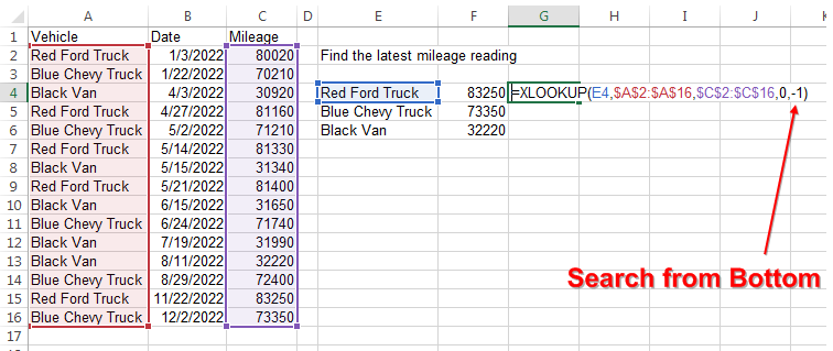
Find the Last Match
XLOOKUP allows you to begin your search at the bottom of the data set. This is great for finding the last match in a data set.
Look to the Left
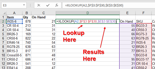
Like LOOKUP and INDEX/MATCH, there is no hassle looking to the left of the key with XLOOKUP.
Where you would have used =INDEX($E$3:$E$30,MATCH(A2,$F$3:$F$30,0)) previously, you can now use =XLOOKUP(A2,$F$3:$F$30,$E$3:$E$30)
Speed Improvements of XLOOKUP
In the example above, the VLOOKUP has to recalculate if anything in the lookup table changes. Imagine if your table included 12 columns. With XLOOKUP, the formula will only recalc if something in the lookup array or results array changes.
In late 2018, the VLOOKUP algorithm changed for faster linear searches. The XLOOKUP maintains the same speed improvements. This makes the linear and binary search options nearly identical. Joe McDaid says there is no significant benefit to using the binary search options in Search_Mode.
Wildcard Support, but Only When You Request It
Every VLOOKUP supported wildcards, making it hard to look up Wal*Mart. By default, XLOOKUP will not use wildcards. If you want wildcard support, you can specify 2 as the Match_Mode.
Multiple Columns of XLOOKUP
Need to do 12 columns of XLOOKUP? You could do it one column at a time...

Or, thanks to Dynamic Arrays, return all 12 columns at once...

Approximate Lookups No Longer Have to Be Sorted
If you need to find the value just less than or just greater than the lookup value, the tables no longer have to be sorted.

Or to find the next larger value:
The Only Disadvantage: Your Co-Workers Won't Have It (Yet)
Due to the new policy of Flighting, only some small percentage of Office Insiders have the XLOOKUP feature today. It could be a while until the function is widely available and even then, it will require an Office 365 subscription. (Dynamic Arrays have been out since September 2018 and still have not rolled out to General Availability.)
Watch Video
Title Photo: Henry Hustava on Unsplash
