Tables Are Like a Database in Excel
May 30, 2022 - by Bill Jelen

Problem: Excel isn’t like Access. I am an Access person and Excel annoys me.
Strategy: If you have database-like data in Excel, define the data as a table.
Many spreadsheets in Excel contain a two-dimensional table of data. You have headings in the first row, and each row of the worksheet represents a different record in a table.
Because a common task in Excel is dealing with tables, Excel has added several features for dealing with tables. One of the best benefits of the table functionality is that charts and pivot tables based on a table will automatically grow with the table.
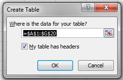
To turn on the features, select a single cell in the dataset and press Ctrl+T. Excel will assume your table extends to either the edge of the spreadsheet or to a blank row and blank column. The Create Table dialog will ask you to confirm the range for the table and that the first row contains headers.

When you apply a table, you will notice the following features:
- Excel applies a default table formatting. You can change to another style using the Table Styles gallery on the Table Tools Design tab.
- Excel turns on the Filter dropdowns on each heading. You can use these dropdowns to sort by a column or to filter a column.
- If you are in the table and scroll so the headings are not visible, the headings will replace column letters A, B, C and so on. The Filter dropdowns will remain available after the first row scrolls out of view.
- You can add totals to the bottom of the dataset by using the Total Row check box in the Table Tools Design tab.
The following features are not immediately visible, but will work:
- Any new data typed in the blank row below the table will be made part of the table. This means that any charts, pivot tables, or formulas that refer to the table will automatically apply to the new data.
- A resize handle in the bottom-right corner of the table allows you to drag to manually extend the table to include additional columns.
- You can use the Table Style Options check boxes to turn on alternate formatting for the first column, last column, header row, total row, or to apply alternating shading to rows or columns.
- Any formulas that point to columns in the table will be written in a new table nomenclature. Enter a formula once and Excel will copy it to all rows of the table.
Gotcha: the filter dropdowns cover up some of the headings. You will find that you end up left-aligning headings so that you can read the headings. You can turn off the filter dropdowns by using Data, Filter.
Gotcha: sometimes you turn on the table functionality to quickly apply a format to the table. It is okay to use Ctrl+T to create and format a table and then immediately use Table Tools, Convert to Range to turn the table back into a normal range. The table formatting remains!
Additional Details: For more information on table, check out the book Excel Tables by Zack Barresse and Kevin Jones.
This article is an excerpt from Power Excel With MrExcel
