Summarize Data with Pivot Tables

Learn Excel from MrExcel Podcast, Episode 2191: Summarize with a Pivot Table.

This is wrapping up our Summarized Data Week-- five different methods to create a summary report of one line per Customer. And Pivot Tables-- why didn't I do this first? Well, that's a great question.

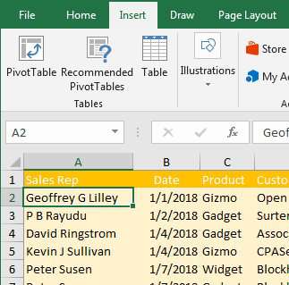
So here we have our original data set. Choose one cell on the data, Insert, Pivot Table, just accept all of these defaults, click OK. We got a brand new worksheet to the left of the original worksheet. This is where the report's going to be built, and it's going to be… choose Customer, sends it to the rows area. Quantity, Revenue, Profit, and Cost. On a bigger screen I would have had to scroll. I think nine clicks, and there is our result. Definitely the fastest, easiest, coolest way to go out of the whole week.

Now, all five methods that we talked about this weak are in this book, MrExcel 54-- LIVe, Live. MrEcel LIVe, The 54 Greatest Excel Tips of All Time. Click that "I" on the top right-hand corner.

All week we take a look at how to create this report five different ways: Subtotals, Remove Duplicates, Advanced Filter, Consolidate, and then today, Pivot Tables. It's easy; it's nine clicks. Select one cell in your data, Insert, Pivot Table, OK, and then in the Pivot Table field list just add a check mark to Customer, Quantity, Revenue, Profit, and Cost; and that's it, nine clicks you're done. Tomorrow, we're going to wrap up with these-- a summary of these five methods and a chance for you to vote on your favorite.

Want to thank you for stopping by, we'll see you next time for another netcast from MrExcel.